In Google Sheets, you can use SUMIF formula to SUM current week’s data. But to make the SUMIF formula to work, you should use the ArrayFormula together with it. Why? It’s because we want to use the WEEKNUM function as the Criterion in SUMIF which is not an array formula by default.

Reference: Google Sheets Functions Guide

As said above, the SUMIF formula can sum a column based on week number in another date column. But don’t think that this’s the only formula that can use for the same purpose. You can also use formulas based on the functions Filter, Query, and SUMPRODUCT for this.

In this tutorial, you can learn how to use SUMIF formula to sum current week’s data. Also, I’ll explain the use of SUMIFS with multiple conditions similarly. Here we go.

How to Use SUMIF Formula to SUM Current Week’s Data

We can get the week number of a date with the help of the function WEEKNUM. See this example.

Must Read: Learn All Available Date Functions in Google Sheets

=WEEKNUM("13/07/2018")

If the date in the above formula is entered in A1, the formula would look like this.

=WEEKNUM(A1)

To get the current Week’s Number, you can use the formula as below.

=WEEKNUM(today())

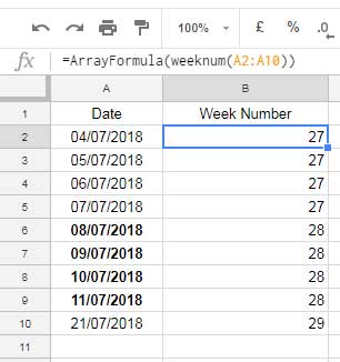
But this’s not an array formula that means it won’t work with dates in a range. But you can make it an Array Formula by using the function ArrayFormula as below.

If you understand this, then you can easily code the SUMIF formula. Now let’s see how to use SUMIF formula to sum current week’s data in Google Sheets.

The SUMIF Formula to SUM Current Week’s Data in Google Sheets

To understand this formula first see the SUMIF syntax.

SUMIF(range, criterion, [sum_range])

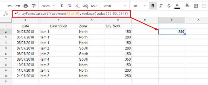
Here is the formula that we’ve used in the above example (it’s already there on the screenshot).

=ArrayFormula(sumif(weeknum(A2:A10),weeknum(today()),D2:D11))

Explanations to the SUMIF function arguments and its use in the formula above.

1. Range: In our sample data, the range A2: A10 contains dates, what we want is week numbers. So the range A2: A10 is wrapped by the WEEKNUM function.

2. Criterion: We can put the current week’s number straight away. If you want to make it flexible, you can extract the week number from today’s date and that’s what I’ve done.

3. Sum_Range: It’s the range to SUM.

You can use SUMIFS in the same way.

How to Use SUMIFS to SUM Current Week’s Data

When you have multiple criteria, use SUMIFS. Here I am not going to the detail section. Just see one formula that using the above sample data.

=ArrayFormula(sumifs(D2:D10,weeknum(A2:A10),weeknum(today()),C2:C10,"North"))

That’s all. Enjoy!

Similar Reading:

1. How to Calculate the Moving Sum of Current Week in Google Sheets.

2. The Formula to Sum by Current Week in Google Sheets.

3. How to Find Current Month’s Week Number In Google Sheets.

4. Find the Date or Date Range from Week Number in Google Sheets.