Most Excel users rely on basic arithmetic operators—addition and multiplication—to calculate the Weighted Moving Average (WMA). But what about Google Sheets users?
In addition to these basic operators, Google Sheets offers more advanced options. You can use the SUMPRODUCT and SUM combo (also available in Excel) or the AVERAGE.WEIGHTED function to calculate the Weighted Moving Average in Google Sheets.
What’s the Purpose of Calculating WMA?
You can find extensive explanations online about the purpose of WMA calculations. However, to keep this tutorial focused, here’s my quick take:
WMA is primarily used by traders. They calculate the Weighted Moving Average and plot charts based on it to generate trade signals, which help in making buying or selling decisions.
Why Use WMA Over SMA?
Before diving into the functions for calculating the Weighted Moving Average (WMA) in Google Sheets, let’s first understand how it differs from the Simple Moving Average (SMA).
SMA (Simple Moving Average):
This is the average of subsets within a dataset. For example, in a 12-month dataset, the SMA could be calculated as the average for every three months.
The key characteristic of SMA is that it gives equal weight to all values in the subset.
Equal weights? What does that mean?
In SMA, you calculate the average by summing all the data points in the subset and dividing by the number of points. For example, if there are 3 data points in the subset, you sum them up and divide by 3. Alternatively, you can use the AVERAGE function directly instead of performing the summing and counting manually.
WMA (Weighted Moving Average):
In contrast, WMA assigns different weights to data points in the subset. More recent data points often have higher weights to reflect their importance. All subsets must follow the same weighting scheme.
Note: For a deeper understanding of WMA, you may want to research further, as I’m not a statistician.
Calculating Weighted Moving Average in Google Sheets
As mentioned earlier, you’ll learn three different methods—or formula options—to calculate the Weighted Moving Average (WMA) in Google Sheets.
1. Using the AVERAGE.WEIGHTED Function
Here, we’ll use sample data. Additionally, we’ll assign weights such as 0.6, 0.3, and 0.1 (placed in cells F5, F4, and F3, respectively).
Formula in cell D5 (copy-paste to D6:D8):
=AVERAGE.WEIGHTED(B3:B5, $F$3:$F$5)- The range reference for the data points (e.g.,
B3:B5) must be relative (without dollar signs). - The range reference for the weights (e.g.,
$F$3:$F$5) must be absolute (with dollar signs).
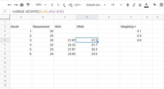
The WMA value in D8 (23.5) represents the weighted moving average for the 7th month.
This is the simplest way to calculate the Weighted Moving Average (WMA) in Google Sheets.
2. Using the SUMPRODUCT Function
An alternative is to use the SUMPRODUCT function. This method is widely used by Excel users.
Replace the formula in D5 with:
=SUMPRODUCT(B3:B5, $F$3:$F$5) / SUM($F$3:$F$5)Copy-paste this formula down the column to calculate WMA for other subsets.
3. Using Basic Arithmetic Operators
If you’re unfamiliar with Google Sheets functions, you can use basic arithmetic operations for the same calculation.
Formula in D5:
=((B3*$F$3)+(B4*$F$4)+(B5*$F$5))/($F$3+$F$4+$F$5)Here too:
- The data points are relative (e.g.,
B3), while the weights are absolute (e.g.,$F$3).
This ensures that the formula adjusts correctly as you drag it down the column.
Plotting SMA and WMA Charts in Google Sheets
Follow these steps to create SMA and WMA charts in Google Sheets:
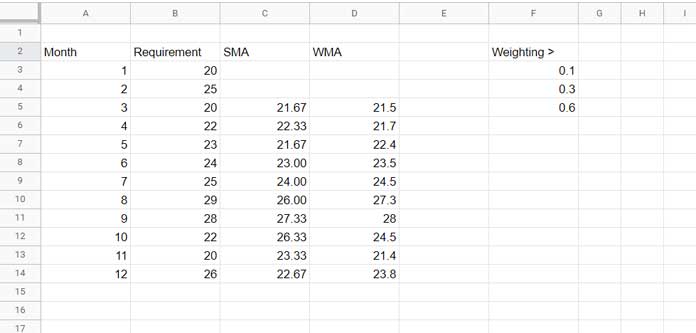
- Select the range A2:D14. Click A2, hold the Shift key, and click D14.
- Right-click the selected range and choose Copy.
- Paste the copied data into A16:D28 using Paste Special > Paste values only.
- Select A16:D28 again and copy it.
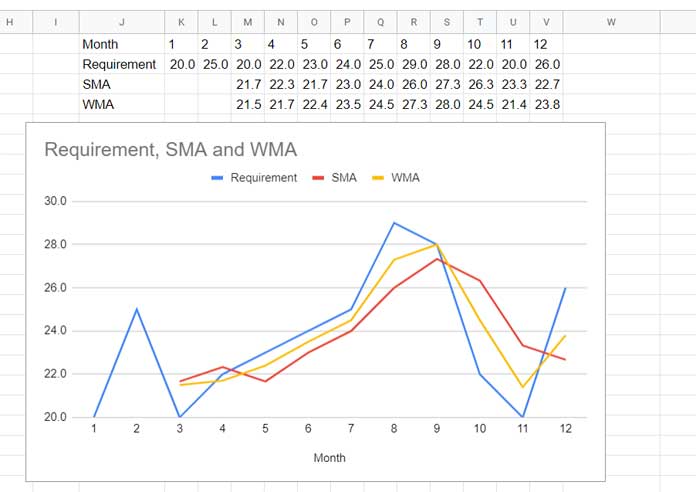
- Paste the transposed data into J1:V4 using Paste Special > Paste transposed.
- Delete the data in A16:D28 (as it’s no longer needed).
- Select J1:V4.
- Go to Insert > Chart and select a Line chart.
This will create a combined SMA and WMA chart in Google Sheets.
Related: Weighted Average of Filtered (Visible) Data in Google Sheets


