Let me shed some light on how to count columns in a row from the first non-blank cell to the last non-blank cell in Google Sheets. Yes! I am back with yet another useful and clever Google Sheets formula.
For example, I have one value in cell H2 and another in cell L2. It can be any values like special characters, strings, dates or numbers.
The cells C2, D2…G2 (C2:G2) are blank and also there is no value from the cell M2 onwards in that row.
I want a formula to return # 5 as the count (H2, I2, J2, K2, and L2) in cell B5 counting the row C2:N2 or more conveniently an infinite range C2:2.
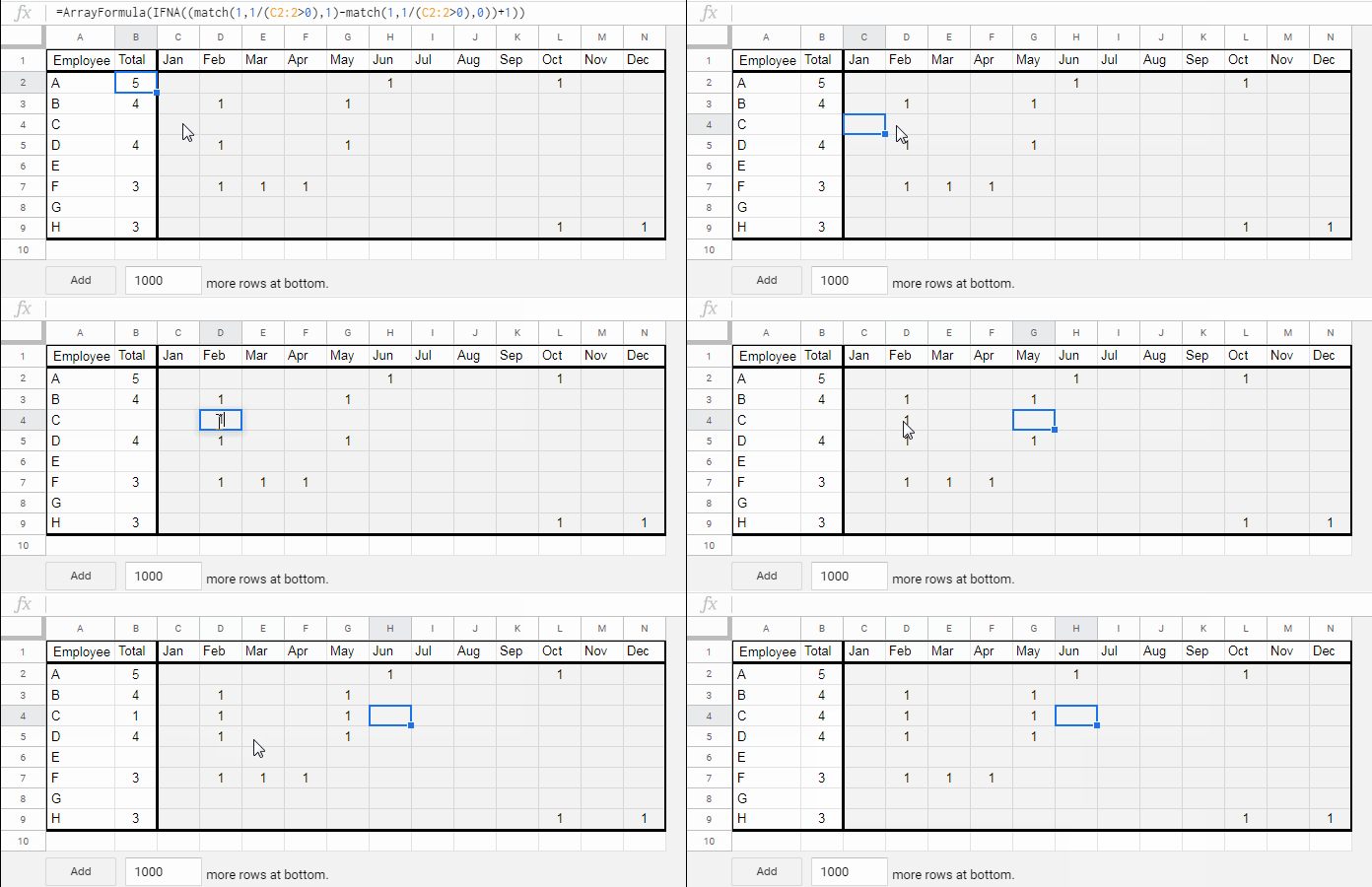
Hope you could understand what I am trying to say. If not, please see the GIF screenshot below. The formula is in the range B2:B9.

Let me share with you the clever formula that helps me count columns in a row skipping blank cells at the beginning and end of a range in Google Sheets.
You can test it with your own sample data by changing some of the cell references in the formula. I’ll explain that later.
In my above example, cell B2 contains the following formula that returns the count from the first non-blank cell H2 to the last non-blank cell L2.
Formula to Count Columns in a Row Skipping Blank Cells at the Beginning and End
Formula:
=ArrayFormula(IFNA((match(1,1/(C2:2>0),1)-match(1,1/(C2:2>0),0))+1))This formula has been copied to B3:B9. Let me elaborate on how this formula returns the count of columns skipping blank cells at the beginning and end. Before that here is how to modify this formula for your range.
Formula Customization:
The above formula is to count from the first non-blank cell C2 to last no-blank cell in the row, not N2.
That means the formula looks the entire range C2:2 (not C2:N2) for the last non-blank cell.
Note: If you don’t understand the range C2:2 enter it as =C2:2 in the 4th row (in any row other than the 2nd row) of your Spreadsheet. It will highlight the said range.
To limit the range to a specific column you can adjust the range like C2:N2 in the formula.
It’s not an expanding formula. Want the count from the first non-blank cell to the last non-blank cell in other rows?
If so, you must copy-paste the formula to the required cells down (in column B).
I hope you will be able to adjust/customize the formula as per your Google Sheets table now.
How the Formula Returns the Count From First Non-Blank Cell to Last Non-Blank Cell?
This is the formula explanation/logic section. It involves two important points.
- A formula that counts the numbers of cells up to the last non-blank cell.
- Another formula that counts the number of cells up to the first non-blank cell.
I can relate these two points in a Generic Formula as below.
Count From First Non-Blank Cell to Last Non-Blank Cell = Point # 1 Formula – Point # 2 Formula + 1
Here are those two formulas.
Point # 1 Formula:
=ArrayFormula(match(1,1/(C2:2>0),1))This formula already featured/explained here – Find the Last Non-Empty Column in a Row in Google Sheets.
Point # 2 Formula:
=ArrayFormula(match(1,1/(C2:2>0),0))This is the same as the Point # 1 formula except for the Match function last argument (search_type).
It is 1, means sorted range, in Point # 1 formula. Here it is set to 0, which means the range is not sorted.
MATCH(search_key, range, [search_type])In cell B2, I have combined these two formulas as per the Generic formula above.
When combining multiple formulas, as I have explained many times, in almost all cases, you can use one single ArrayFormula, instead of using multiple ones.
In the combination, additionally, I have used IFNA to skip N/A errors in totally blank rows.
Formula Logic:
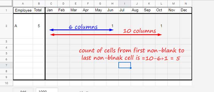
I know a few of you may want to know the formula logic.

I hope the above image will well explain the same.
Additional Resources:


