How to Count Orders per Week in Google Sheets: Formula Examples

To count orders per week in Google Sheets, you can utilize either the WEEKNUM or WEEKDAY date functions along with QUERY. This tutorial covers both functions to help you:

Determine the number of requests/orders received per week or individually for each week.
Calculate the count of orders placed each week.

If you opt for the WEEKNUM function, the summary will be based on week numbers. Conversely, the WEEKDAY function generates calendar weeks, like 28/Jan/19 – 03/Feb/19, instead of the week number (e.g., 5 for this week).

This Google Spreadsheets tutorial provides both solutions, and I’ve also included instructions on using IMPORTRANGE. This is particularly useful if your source data, i.e., the recorded dates, is in one sheet, and you want week-wise counts in another sheet.

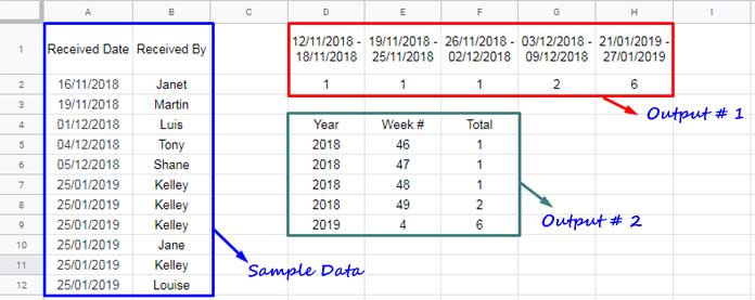
Follow the steps outlined in the tutorial, including sample data in cells A2:B. The screenshot illustrates two types of outputs, and I’ve included formulas for both. Choose the one that best fits your needs.

For a hands-on experience, you can access my Demo Sheet with Formulas.

Sample Sheet

How to Count Orders Per Week Using Week Numbers in the QUERY Function

Output #2 Method (Refer to the screenshot above):

In the (output #2 method), I utilized week numbers to represent the count of orders per week. Consequently, the WEEKNUM function, combined with QUERY, enables the tracking of order receipts on a week-by-week basis.

Now, let’s delve into the specifics of how to count orders per week in Google Sheets.

Referring to the provided example, I’ve placed the formula in cell D4. Let’s break down the step-by-step process of developing that formula.

a. How to Extract Week Numbers and Years from Dates

While the QUERY function doesn’t have the WEEKNUM scalar function, it does include the YEAR function. To extract week numbers from dates and horizontally stack them with the date, we’ll use the native WEEKNUM date function.

Formula #1: Enter in cell D2.

=HSTACK(A2:A, ARRAYFORMULA(WEEKNUM(A2:A,2)))

The source data starts from row #2, so input this formula in cell D2.

The following WEEKNUM array formula extracts week numbers from the dates in A2:A.

=ARRAYFORMULA(WEEKNUM(A2:A, 2))

I have considered Monday-Sunday as the calendar week, indicated by the number 2 inside the WEEKNUM formula. If you prefer Sunday-Saturday, change that number to 1.

Note that blank cells are treated as 0, and if formatted as dates, they will display as 30/12/1899. Consequently, the formula may return 53 for blank cells. This is not an issue, as we will filter out those blank rows in the QUERY.

Concerning the year, there’s no need to separate it from the date, as we can achieve that within QUERY using the YEAR scalar function.

We will use the above formula #1 as data in QUERY to return the count per week using Week Numbers.

b. Using QUERY to Group Week Numbers and Years with Count Aggregate Function

We can use the above formula output as the source data in QUERY. It’s a two-column dataset. Count any of the columns and group them by year and then by week number. Here is that formula.

Formula #2 (Master Formula): Modify the existing formula in cell D2

=LET(dt, A2:A, QUERY(
     HSTACK(dt, ARRAYFORMULA(WEEKNUM(dt, 2))), 
     "SELECT YEAR(Col1), Col2, COUNT(Col1) 
     WHERE Col1 IS NOT NULL 
     GROUP BY YEAR(Col1), Col2 
     LABEL YEAR(Col1) 'Year', Col2 'Week #', COUNT(Col1) 'Total'", 
     0
))

Note: Instead of HSTACK(A2:A, ARRAYFORMULA(WEEKNUM(A2:A,2))), we have used HSTACK(dt, ARRAYFORMULA(WEEKNUM(dt,2))) because we utilized the LET function, assigning the name dt to the range A2:A.

This formula adheres to the following QUERY syntax:

QUERY(data, query, [headers])

Where:

data: HSTACK(dt, ARRAYFORMULA(WEEKNUM(dt, 2)))

query: "SELECT YEAR(Col1), Col2, COUNT(Col1) WHERE Col1 IS NOT NULL GROUP BY YEAR(Col1), Col2 LABEL YEAR(Col1) 'Year', Col2 'Week #', COUNT(Col1) 'Total'"

SELECT YEAR(Col1): Extracts the year from the first column (original date column).
Col2: Represents the second column, which is the week number generated.
COUNT(Col1): Counts the occurrences of each unique combination of year and week number.
WHERE Col1 IS NOT NULL: Ensures that only non-null values in the date column are considered.
GROUP BY YEAR(Col1), Col2: Groups the data by year and week number.
LABEL YEAR(Col1) 'Year', Col2 'Week #', COUNT(Col1) 'Total': Provides custom labels for the output columns.

header: 0

This is the second output method to count orders per week in Google Sheets.

How to Count Orders Per Week Using Weekday in QUERY

Output #1 Method (Refer to the screenshot above):

Here is an alternative solution to count orders per week in Google Sheets. In this approach, two formulas are required: one for the column names (field labels) and the other for generating the count.

a. Creating Week-Wise Column Names in Google Sheets

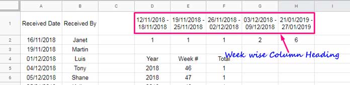
In a recent Google Sheets tutorial, I detailed how to generate calendar weeks’ start and end dates as column names instead of week numbers, employing a combination of the WEEKDAY function to achieve this.

Here, I am going to use a slightly improved (modernized) version of that formula directly without explaining. If you are interested in understanding this formula, you can refer to my tutorial titled “Calendar Week Formula in Google Sheets to Combine Week Start and End Dates.” However, this is not a prerequisite, as I can guide you on modifying the formula range to suit your data range.

Formula #3 (Master Formula 1):

=ArrayFormula(LET(
     dt, A2:A, 
     wd, WEEKDAY(DATEVALUE(dt), 2), 
     TOROW(
          TEXT(SORT(UNIQUE(TOCOL(dt - wd + 1, 3))), "DD/MM/YYYY") &" - "& 
          TEXT(SORT(UNIQUE(TOCOL(dt - wd + 7, 3))), "DD/MM/YYYY")
     )
))

In my example, I have entered the above formula in cell D1, where it populates the column names.

The above formula is designed for our receipt dates in A2:A. If your data range is different, simply change the reference A2:A in the formula. Another adjustment you may need is the date formatting, currently set as “DD/MM/YYYY”. Feel free to modify this to “MM/DD/YYYY” if you prefer.

Similar to formula output #1, I have considered Monday-Sunday as the calendar week, indicated by the 2 (type) used in the WEEKDAY formula. If you prefer Sunday-Saturday, change that number to 1.

b. Week Wise Count in Google Sheets

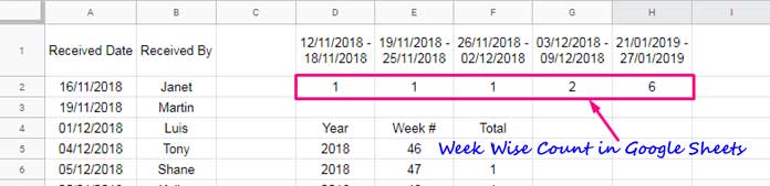
Now, we want the formula to count orders per week for the provided date range in the heading. For that purpose, we can utilize the previously mentioned Formula #2 (Master Formula) with a modification.

The mentioned formula returns a three-column output: “Year”, “Week #”, and “Total” as the column names (heading).

In this case, we only want the last column (Total) from that output without the column name/label. Additionally, we need to transpose the result.

Here is the formula that you can use in cell D2.

Formula #4 (Master Formula 2):

=TOROW(LET(dt, A2:A, QUERY(
     HSTACK(dt, ARRAYFORMULA(WEEKNUM(dt,2))), 
     "SELECT COUNT(Col1) 
     WHERE Col1 IS NOT NULL 
     GROUP BY YEAR(Col1), Col2 
     LABEL COUNT(Col1) ''", 
     0
)))

That’s all. Using either of the two output methods, you can count orders per week in Google Sheets.

Counting Orders Per Week Using Imported Data

Can I use the above methods between two Google Sheets files?

Yes! Suppose your daily entry (source data) is in the file “receipt order”. You want to generate the weekly count summary in another file called “weekly summary”.

In that case, you can use the IMPORTRANGE function to import the data into the “weekly summary” file. Here are the steps involved.

Here, you can also apply the above two methods.

Output #2 Method (Week Number Wise Summary)

Steps:

First, enter the following IMPORTRANGE formula in any cell in row #2 in your “weekly summary” file:

Formula #5:

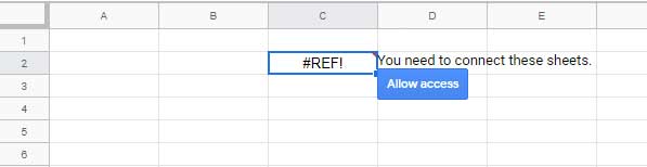
=IMPORTRANGE("URL", "Sheet1!A2:A")

In this formula, replace “URL” with the URL of your “receipt order” file and the sheet name with the tab name that contains the source data. If you encounter a #REF! Error, allow access.

Now scroll to the top of this page and copy the formula given under “Formula #2 (Master Formula)”.

Replace the cell references A2:A in that formula with the above IMPORTRANGE formula. It should look something like this:

Formula #6 (Master Formula):

=LET(dt, IMPORTRANGE("URL", "Sheet1!A2:A"), QUERY(
     HSTACK(dt, ARRAYFORMULA(WEEKNUM(dt, 2))), 
     "SELECT YEAR(Col1), Col2, COUNT(Col1) 
     WHERE Col1 IS NOT NULL 
     GROUP BY YEAR(Col1), Col2 
     LABEL YEAR(Col1) 'Year', Col2 'Week #', COUNT(Col1) 'Total'", 
     0
))

If you have done everything correctly, it should return the correct week number-wise count. This means Output #2 is successfully counting orders per week using imported data in Google Sheets.

Output #1 Method (Calendar Week Start and End Date Wise Summary)

In this method, please copy the formulas “Formula #3 (Master Formula 1)” and “Formula #4 (Master Formula 2)” and change the cell reference A2:A with the IMPORTRANGE formula.

I am not repeating those formulas here. If you follow the above tutorial carefully, you can easily create this type of weekly summary count in Google Sheets.

That’s all. Enjoy!

Resources

Here are some guides that discuss the usage of week numbers in various formulas in Google Sheets.

26 COMMENTS

Chris January 29, 2024 At 9:25 pm

Thanks Prashanth, your help with this would be fantastic as I’m getting a little lost with the formulas! 🙂 I will email you an example sheet and hopefully you can work your magic to make the formula work the way I am hoping it might.

- Prashanth KV February 1, 2024 At 8:52 am
  
  It seems I accidentally deleted your email, or I couldn’t find it. Could you please provide the URL in your reply below? I assure you that it will be kept unpublished.
  
- Prashanth KV February 20, 2024 At 8:25 am
  
  I’ve responded to your email today. Kindly review the formulas in your sheet. The formula employs the “Convert Dates to Week Ranges in Google Sheets (Array Formula)” approach, which you can locate under the “Resources” section above.
  
Chris January 17, 2024 At 11:47 pm

Thanks, Prashanth. Does that mean I will have to use a pivot table? I’m hoping to avoid this if possible.

- Prashanth KV January 18, 2024 At 9:41 am
  
  Nope! In one tutorial, I’ve explained a formula that you can use in a helper column alongside your table. You can use that column to group and sum or apply whatever aggregation you want in your QUERY.
  
  In the Pivot Table tutorial, I’ve included a tip to use the above formula to adjust according to your specific week start and end.
  
  If you’d like, you can share an example sheet with me.
  
Chris January 16, 2024 At 10:43 pm

Hi,

To record the number of requests (under a selection of different categories) that our service receives per week, I’m using your Formula #4 (Master Formula 2) for each different category.

Is there a way to add to the above formula so that if there are no items (in this case requests) recorded in any given week, it then shows as 0 (zero)?

- Prashanth KV January 17, 2024 At 12:33 pm
  
  It seems you may have missed my recent tutorials. Please check out the last two tutorials under “Resources” in this guide.
  
Andy R July 6, 2023 At 6:14 pm

Great tutorial! However, I seem to be getting multiple duplicate dates using option 1. I believe this is because I am using a full timestamp rather than just a date. I can’t seem to figure out how to adjust the code to ignore the time part of the stamp. Any help would be appreciated.

- Prashanth July 7, 2023 At 11:21 am
  
  Hi Andy R,
  
  To get the date from a timestamp, use the INT function. Please see the sheet “User Requested 2” in my shared sample file. You can find the file in the above tutorial.
  
  - Andy R July 7, 2023 At 2:03 pm
    
    Thank you so much! I completely missed the sample file. I appreciate you pointing that out and for this great tutorial. Keep up the good work!
    
JayS June 29, 2023 At 12:49 am

Hi,

In your above example, you have a column that indicates whether an order has been approved, not approved, or cancelled. I am using Output #1 and want to remove the items from the count that have been cancelled. How can I do that? Please let me know.

Thanks

- Prashanth June 29, 2023 At 1:24 pm
  
  Hi JayS,
  
  Please see the tab named “User Required” in my shared example sheet above.
  
  - JayS June 29, 2023 At 6:35 pm
    
    Hello Prashanth,
    
    Thanks for your help! Is it possible to do the same thing, but with a column that says “Approved” or “Cancelled” instead of assigning them numbers? The dataset I’m working with has thousands of entries, and numbering each one would be very time-consuming.
    
    Thanks again for your help!
    
    - Prashanth June 29, 2023 At 9:25 pm
      
      Done!
      
GBF TeachSTEM March 30, 2023 At 11:29 pm

Hi,

I could use the formula to automatically count the number of entries coming (“Raw Responses” tab) for a given week.

How do I get the count of cleaned applications (“Cleaned Applications” tab) in another tab alongside the above count?

Any help in understanding the query formula would be great!

Here is the sample sheet: removed by admin

- Prashanth March 31, 2023 At 2:33 pm
  
  Hi, GBF TeachSTEM,
  
  It requires a different kind of formula which I’ve added to your sample Sheet. The tab name is “Infoinspired.”
  
Kar February 4, 2022 At 12:13 am

Is there a way to get output 2 to go vertically instead of horizontally? Just a bit better for spacing for me. Thanks!

- Prashanth February 5, 2022 At 9:34 am
  
  Hi, Kar,
  
  Output # 2 is already aligned vertically.
  
  I guess you are referring to the output # 1 method. Then remove the Transpose from the following two formulas.
  
  1. Formula # 3 (Master Formula 1).
  2. Formula # 4 (Master Formula 2).
  
lauren January 29, 2021 At 1:29 am

My data set has blank cells in column 2, but those blank cells are still counted. How do get a true count with blank cells omitted?

- Prashanth January 29, 2021 At 8:34 am
  
  Hi, Lauren,
  
  It’s because I haven’t included the data in B2:B anywhere in the formula. So just included it within the formula.
  
  Here is the updated formula as per “Output # 2 Method”:
  
  =query({sort(if(len(A2:A),{year(A2:A),weeknum(A2:A,2)},),1,true,2,true),B2:B},"Select Col1,Col2, Count(Col1) where Col3 is not null group by Col1,Col2 label Col1'Year', Col2'Week #',Count(Col1)'Total'",0)
  
  There are two changes.
  
  1. The range B2:B included in the formula.
  2. Replaced the Query Where clause where Col is not null with where Col3 is not null.
  
  This will help you to omit the rows in the count wherever column B has no value.
  
NurseBuck November 3, 2020 At 9:43 pm

So, using your formula, can you add a Countif string so that the weekly totals reference a certain word being present in a column?

For example, if I wanted to see how many times the word “positive” was present in Cell G2:G using your weekly totals formula, what would I add to the formula?

- Prashanth November 5, 2020 At 4:46 pm
  
  Hi, NurseBuck,
  
  This may help.
  
  Conditional Week Wise Count in Google Sheets.
  
Brad Larsen Sanchez October 13, 2020 At 3:25 am

Similarly, once I have the week number for a range of dates spanning all of 2020, how can I sum the number of “sales” per week and sort by the salesperson assigned to the sale?

A1 = Date of Service
A2 = Week Number of Year
A3 = Sales Person Name

I want to count the number of sales per salesperson per week.

- Prashanth October 16, 2020 At 10:45 am
  
  Hi, Brad Larsen Sanchez,
  
  Assume the data range is A1:C and A1:C1 contains the labels.
  
  Then try either of the below two Query formulas.
  
  Only Grouping:
  
  =query({A1:C},"Select Col3,Col2, count(Col2) where Col2 is not null group by Col3,Col2",1)
  
  Grouping and Pivot:
  
  =query({A1:C},"Select Col3, count(Col3) where Col2 is not null group by Col3 pivot Col2",1)
  
Pushpkant Garg June 17, 2020 At 10:21 pm

How can I get data week-wise for items? For Example, I have a data sheet as follows.

Date | Item
1/1/2020 | Mango
1/1/2020 | Apple
10/1/2020 | Mango

The result I want is;
Week | Mango | Apple
Week 1 | 1 | 1
Week 2 | 1 | 0

How can I achieve this solution?

- Prashanth June 18, 2020 At 12:08 pm
  
  Hi, Pushpkant Garg,
  
  Since you have not given the cell-range of your data, let’s consider it as A1:B. If, so try the below Query in cell C1.
  
  =ArrayFormula( query( {"Week "&weeknum(A2:A),B2:B}, "Select Col1, count(Col1) where Col2 is not null group by Col1 pivot Col2 label Col1'Week'" ) )
  
  Best,