When you need to create a conditional week wise count in Google Sheets, the QUERY function can be a powerful tool.
If no condition is required, you can choose from QUERY, COUNTIF, or COUNTIFS:
- COUNTIF works if you don’t want to include the year part in the week-wise summary.
- COUNTIFS is the better option when you want to include the year in the summary.
- QUERY is versatile and works in all cases.
In this tutorial, you’ll learn how to use the QUERY function for a conditional week-wise count in Google Sheets.
To make the concepts clear, I’ll also briefly show how COUNTIF and COUNTIFS handle week-wise counts.
Sample Data for Testing
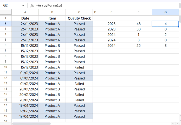
We’ll use the following basic production data to demonstrate the formulas.

Try it yourself: Open this sample Google Sheet to follow along with the formulas in this tutorial.
COUNTIF for Week Wise Count (Without Conditions)
If you just want to count items week-wise without conditions, COUNTIF can work.
Steps:
- In cell
E2, enter this formula to get the unique week numbers:=ArrayFormula(UNIQUE(IF(A2:A="",,WEEKNUM(A2:A))))
(This formula extracts the week numbers from the Date column.) - In cell
F2, use:=ArrayFormula(IF(E2:E="",,COUNTIF(WEEKNUM(A2:A), E2:E)))
Note: By default, WEEKNUM in Google Sheets considers weeks as Sunday–Saturday. To start weeks on Monday, use WEEKNUM(date, 2).
Limitation:
COUNTIF can only handle one condition in this format. Since the week number is already the condition, you cannot add another condition for a conditional week wise count in Google Sheets.
COUNTIFS for Conditional Week Wise Count
Single Condition – Item
COUNTIFS can handle conditional week wise counts.
Example: Count the weekly occurrences of Product A.
=ArrayFormula(
   IF(E2:E="",,
      COUNTIFS(WEEKNUM(A2:A), E2:E, B2:B, "Product A")
   )
)
Multiple Conditions – Item and Quality Check
To count the weekly occurrences of Product A where the Quality Check is Passed:
=ArrayFormula(
   IF(E2:E="",,
      COUNTIFS(WEEKNUM(A2:A), E2:E, B2:B, "Product A", C2:C, "Passed")
   )
)
Including Years:
Replace the week number formula in E2 with:
=ArrayFormula(UNIQUE(IF(A2:A="",,HSTACK(YEAR(A2:A), WEEKNUM(A2:A)))))Then update the COUNTIFS formula to reference both year and week:
=ArrayFormula(
     IF(E2:E="",,
        COUNTIFS(YEAR(A2:A), E2:E, WEEKNUM(A2:A), F2:F, B2:B,"Product A", C2:C,"Passed")
     )
)
Why Use QUERY for Conditional Week Wise Count?
The QUERY function provides more flexibility and cleaner summaries.
If you’re new to QUERY, see my complete guide to the QUERY function in Google Sheets for syntax and examples.
Although QUERY has no built-in WEEKNUM function, you can generate week numbers using the spreadsheet function and include them in the query data.
Preparing the Query Data – Year and Week Numbers
=ArrayFormula(IF(A2:A="",,HSTACK(YEAR(A2:A), WEEKNUM(A2:A), B2:C)))This creates:
- Column 1: Year
- Column 2: Week number
- Column 3: Item
- Column 4: Quality Check
The formula outputs a table like this (only the first few rows shown):
| Year | Week Number | Item | Quality Check |
| 2023 | 48 | Product A | Passed |
| 2023 | 48 | Product A | Passed |
| 2023 | 48 | Product A | Passed |
| 2023 | 48 | Product A | Passed |
| … | … | .. | … |
QUERY for Conditional Week Wise Count
Example – Counting by Year and Week:
=QUERY(
     ArrayFormula(IF(A2:A="",,HSTACK(YEAR(A2:A), WEEKNUM(A2:A), B2:C))),
     "SELECT Col1, Col2, COUNT(Col1)
      WHERE Col1 IS NOT NULL
      GROUP BY Col1, Col2
      LABEL Col1 'Year', Col2 'Week'"
)
Output:
| Year | Week | Count |
| 2023 | 48 | 4 |
| 2023 | 50 | 5 |
| 2024 | 1 | 3 |
| 2024 | 3 | 3 |
| 2024 | 25 | 3 |
Adding Conditions (Item is Product A and Quality Check = Passed)
=QUERY(
     ArrayFormula(IF(A2:A="",,HSTACK(YEAR(A2:A), WEEKNUM(A2:A), B2:C))),
     "SELECT Col1, Col2, COUNT(Col1)
      WHERE Col3='Product A' AND Col4='Passed'
      GROUP BY Col1, Col2
      LABEL Col1 'Year', Col2 'Week'"
)
Output:
| Year | Week | Count |
| 2023 | 48 | 4 |
| 2024 | 1 | 2 |
| 2024 | 25 | 3 |
Conclusion
For a conditional week wise count in Google Sheets, you can use COUNTIFS for simpler cases, but QUERY is more powerful when:
- You need multiple conditions
- You want year and week in the same summary
- You want a clean table output without helper columns


