Want to visually separate and highlight sections of grouped data in Google Sheets — all with a simple checkbox? You can do that with just one conditional formatting rule. In this tutorial, we’ll see how to highlight multiple groups using checkboxes (tick boxes) in Google Sheets. Each group is independently controlled by the checkbox placed at the top of that group.

This method is perfect for scenarios where your data doesn’t have any category label or identifier. You simply define where a group starts by placing a tick box, and then highlight the entire group based on the ticked status.

How Checkbox-Based Group Highlighting Works

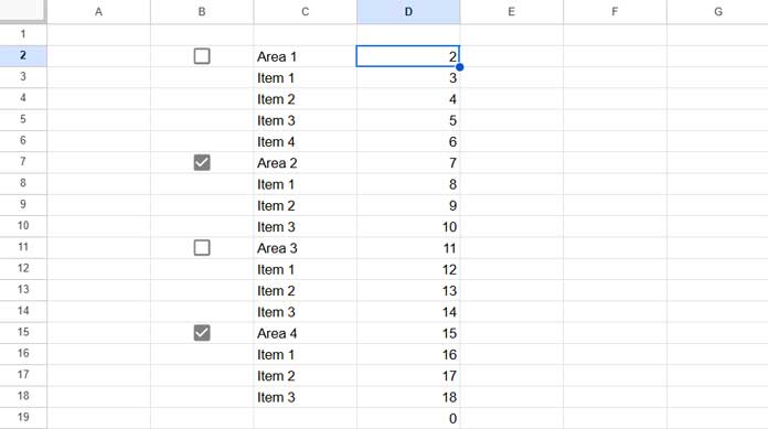
Let’s set up the idea first:

• Column C contains your grouped data.
• Column B contains tick boxes (Insert > Tick box).
• You place the tick box only in the first row of each group.
• Ticking a box highlights the associated group — until the next tick box or end of data.

This setup is ideal for highlighting groupings dynamically without needing a dedicated category column.

Custom Formula to Highlight Multiple Groups Using Checkboxes

Here is the custom formula we’ll use in conditional formatting:

=XMATCH(ROW(C2), ARRAYFORMULA(LET(r, $B$2:$B, tr, ROW(r), XLOOKUP(tr*(tr<=XMATCH("?*", C:C&"", 2, -1)), tr/IF(r<>"", TRUE, FALSE), r, , -1)*ROW(r))))

✅ This works for:

• Checkbox column: B2:B
• Data column (groups): C2:C

How to Apply the Rule

1. Select the data range you want to highlight (e.g., C2:C)
2. Go to Format > Conditional formatting
3. Under Format cells if, select Custom formula is
4. Paste the formula above
5. Choose a formatting style (e.g., background color)
6. Click Done

That’s it! Now each group will be highlighted when its leading tick box is checked.

Adjusting the Formula for Your Sheet

If you’re using a different layout, update the formula as follows:

• Replace C2 with the first cell in your data range
• Replace $B$2:$B with the checkbox range
• Replace C:C with the entire data column

Formula Explanation

Let’s break the formula into logical parts:

=XMATCH(ROW(C2), ARRAYFORMULA(LET(
  r, $B$2:$B,
  tr, ROW(r),
  XLOOKUP(
    tr*(tr<=XMATCH("?*", C:C&"", 2, -1)),
    tr/IF(r<>"", TRUE, FALSE),
    r, , -1
  ) * ROW(r)
)))

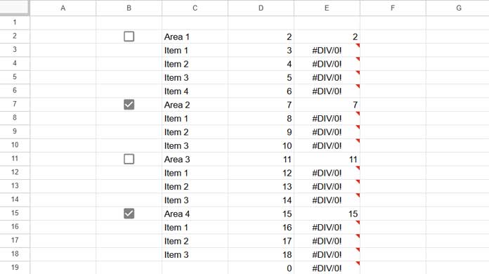
1. XMATCH("?*", C:C&"", 2, -1)

• Finds the last non-blank row in column C.
• The expression tr <= XMATCH(...) ensures we only process rows up to the last entry.

2. tr*(tr <= last_row)

• Generates a numeric array of row numbers from the data range (e.g., 2 to 18), and 0s afterward.

3. tr/IF(r<>"", TRUE, FALSE)

• Creates an array of row numbers only where a checkbox exists.
• In all other rows, it returns an error — which is essential for the next step.

4. XLOOKUP(...)

• This is the clever part:
• It looks up each row number in the array of checkbox rows.
• The -1 match mode tells it to find the last earlier match — effectively filling each group’s rows with the checkbox value from above.

This fill-down logic is covered in more detail in our tutorial: Fill Blank Cells with Values from the Cell Above in Google Sheets

5. Multiply by ROW(r)

• We multiply the result with row numbers again to preserve position.
• We now have an array of row numbers where checkboxes are TRUE (ticked).

6. XMATCH(ROW(C2), ...)

• Finally, we check if the current row’s number exists in that array.
• If yes, the conditional formatting applies — and the row is highlighted.

What You Can Do with This Setup

• Tick a box in column B to highlight the group of rows starting from that tick.
• Untick it, and the highlight goes away.
• Works even if you add new rows or groups — just extend the checkbox column accordingly.

Conclusion

Using checkboxes to control group highlighting offers a flexible way to manage visual sections in your data without relying on helper columns or category labels. With a single conditional formatting rule, you can dynamically highlight multiple groups based on user interaction.

For a broader collection of conditional formatting methods—from beginner-friendly ideas to complex formula-driven approaches—see the Ultimate Guide to Conditional Formatting in Google Sheets, your central resource for all related tutorials.

Additional Reading

Here are some related tutorials you might find helpful:

• Conditional Formatting Based on Data Groups in Google Sheets
• Highlight Groups with Alternating Colors in Excel