Row-wise sorting refers to the process of sorting each row in a 2D array using an array formula in Google Sheets. You can achieve this using the BYROW or REDUCE functions in combination with the SORT function. Although the QUERY function can also accomplish this task, it is less recommended due to its complexity for some users.
Example: Sorting Each Row of a 2D Array
Suppose the source data is in the range B2:E5, and the result should appear in B9:E12.
While it is possible to handle this using a non-array formula (copy-paste or drag-down method), using an array formula is often more efficient, especially when the source data is dynamic (e.g., generated by functions like QUERY).
Non-Array Formula
To sort each row individually, you can use this formula
=TRANSPOSE(SORT(TRANSPOSE(B2:E2), 1, 1))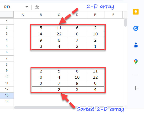
- Insert the formula in B9, and then copy-paste it to B10:B12, or drag the fill handle (blue square in the bottom-right corner) down.
- To sort rows in descending order, replace 1, the last argument in the formula, with 0.
Related: How to Sort Horizontally in Google Sheets.
However, let’s focus on creating an array formula for row-wise sorting and explore the role of the TRANSPOSE function in the process.
Row-Wise Sorting in a 2-D Array: BYROW
The BYROW function is the simplest and most recommended solution for row-wise sorting.
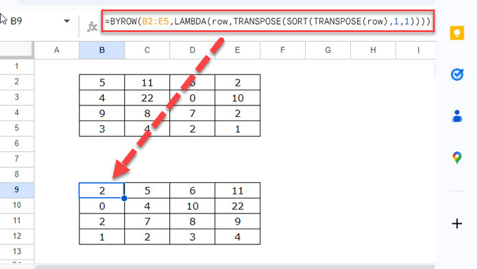
To sort each row of the 2D array B2:E5 in ascending order, use this formula in B9:
=BYROW(
   B2:E5,
   LAMBDA(row,
      TRANSPOSE(SORT(TRANSPOSE(row), 1, 1))
   )
)
To sort rows in descending order, modify the formula:
=BYROW(
   B2:E5,
   LAMBDA(row,
      TRANSPOSE(SORT(TRANSPOSE(row), 1, 0))
   )
)
How the Formula Works
BYROW Syntax:
BYROW(array_or_range, lambda)array_or_range: Refers to the input range (e.g.,B2:E5), which is processed row by row.lambda: A custom function applied to each row.
LAMBDA Syntax:
LAMBDA([name, …], formula_expression)name: Represents the current row (e.g., row).formula_expression: The operation to perform on each row.
In this case:
TRANSPOSE(SORT(TRANSPOSE(row), 1, 1))- The TRANSPOSE function converts the row into a column for sorting.
- The SORT function sorts the transposed column.
- Another TRANSPOSE restores the sorted data to row format.
Using TOCOL and TOROW
To simplify the formula further, you can replace TRANSPOSE with TOCOL and TOROW:
Ascending order:
=BYROW(B2:E5, LAMBDA(row, TOROW(SORT(TOCOL(row), 1, 1))))Descending order:
=BYROW(B2:E5, LAMBDA(row, TOROW(SORT(TOCOL(row), 1, 0))))- TOCOL converts the row into a column for sorting.
- TOROW converts the sorted column back into a row.
This approach avoids using TRANSPOSE twice, making the formula more concise and easier to understand.
Row-Wise Sorting in a 2-D Array: REDUCE
An alternative approach is to use the REDUCE function.
Formula:
=REDUCE(
   TOCOL(,1), SEQUENCE(ROWS(B2:E5)),
   LAMBDA(a, v,
      IFNA(VSTACK(a, TOROW(SORT(TOCOL(CHOOSEROWS(B2:E5, v))))))
   )
)Drawbacks:
- Complexity: The formula is more challenging to write and understand compared to BYROW.
- Performance: While all lambda-based functions are computationally intensive, this approach may be more resource-hungry compared to the BYROW approach due to the repeated use of functions like TOCOL, TOROW, and SORT within the lambda.
How the Formula Works
REDUCE Syntax:
REDUCE(initial_value, array_or_range, lambda)intial_value:TOCOL(,1), nullarray_or_range:SEQUENCE(ROWS(B2:E5)), which generates serial numbers for each row (1 to 4).lambda: A custom function applied iteratively.
LAMBDA Syntax:
LAMBDA([name1, name2], formula_expression)name1:a(the accumulator).name2:v(the current row index)
Formula Breakdown:
IFNA(VSTACK(a, TOROW(SORT(TOCOL(CHOOSEROWS(B2:E5, v))))))CHOOSEROWS(B2:E5, v): Selects the current row.- TOCOL: Converts the row into a column.
- SORT: Sorts the column.
- TOROW: Converts the sorted column back into a row.
- VSTACK: Stacks the sorted row with the accumulator (
a). - IFNA: Handles potential errors, ensuring a valid result.
This process repeats for each row, accumulating the sorted rows into a final array.
Conclusion
Both BYROW and REDUCE can be used for row-wise sorting in a 2D array. While BYROW is simpler and more efficient, REDUCE offers a more advanced, iterative approach.
Choose the method that best suits your needs, and enjoy the flexibility of Google Sheets!


