Discover how to effortlessly group and sum data separated by blank rows in Google Sheets, enhancing your data analysis efficiency.

We typically identify groups in a dataset by using a category column. Summarizing such data is much simpler using functions like SUMIF, SUMIFS, or QUERY in Google Sheets.

However, what if you need to group and sum data separated by one or more blank rows in Google Sheets?

For data aggregation, we usually rely on the mentioned functions, but they require a category column to apply criteria—a component missing when dealing with groups separated by blank rows.

To address this, we’ll automatically assign unique identifiers to each set of data separated by blank rows in Google Sheets. This can be achieved using a formula within Google Sheets itself, eliminating the need for scripting.

I’ve developed a Google Sheets array formula that allocates a unique number to each group, even if an unequal number of blank rows separates them.

Ultimately, we’ll use this assigned column as the category column to effectively group and sum data in Google Sheets.

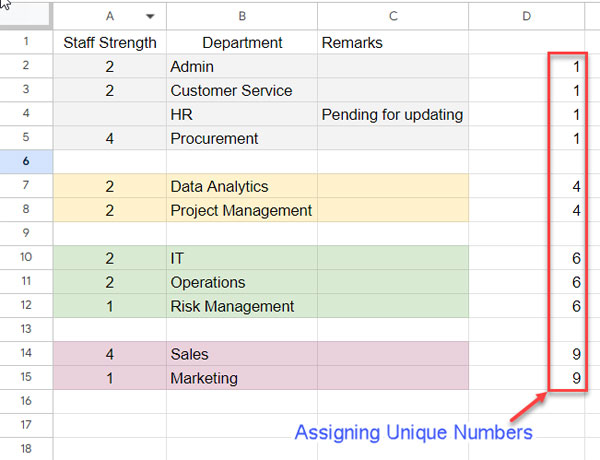
Sample Data and the Problem to Be Solved

In the provided sample data (refer to the screenshot above), staff strength, department, and notes are recorded in columns A, B, and C, respectively.

Rows 6, 9, and 13 are intentionally left blank. The objective is to calculate the total staff strength separately for the following groups: rows 2 to 5, 7 & 8, 10 to 12, and 14 & 15.

Additionally, it’s crucial to note that when identifying blank rows, the entire row in the specified range must be blank; a single blank cell is not considered sufficient for this analysis.

Let’s explore how to group and sum datasets in Google Sheets, where groups are separated by blank rows.

Formula for Grouping Data Separated by Blank Rows in Google Sheets

Given our sample data range in A2:C, you can apply the following formula to cell D2, the top row of the next available column:

=ARRAYFORMULA(LET(data, A2:C, empty, IF(LEN(TRIM(TRANSPOSE(QUERY(TRANSPOSE(data),,9^9))))>0,1,), rc, COUNTIFS(empty, "<>"&empty, SEQUENCE(ROWS(data)), "<="&SEQUENCE(ROWS(data))), test, SCAN(1, rc, LAMBDA(a, v, IF(v=0, a, v))), IF(LEN(empty), test, )))

This formula generates unique numbers to facilitate grouping data separated by blank rows, producing numbers like 1, 4, 6, and 9 for each group.

By utilizing column D or the formula in cell D2 as the category column, you can efficiently number, group, and sum data separated by blank rows in Google Sheets.

Before delving into practical application, let’s break down the components of the formula, providing valuable insights for users seeking to advance their skills in Google Sheets.

Formula Explanation

The formula that groups data separated by blank rows is essentially a LET function that assigns ‘name’ with the ‘value_expression’ and returns the final result of the ‘formula_expression.’

Syntax:

LET(name1, value_expression1, [name2, …], [value_expression2, …], formula_expression)

Where:

• name1 = data
• value_expression1 = A2:C
• name2 is empty
• value_expression2 is IF(LEN(TRIM(TRANSPOSE(QUERY(TRANSPOSE(data),,9^9))))>0,1,)
• name3 = rc
• value_expression3 = COUNTIFS(empty, "<>"&empty, SEQUENCE(ROWS(data)), "<="&SEQUENCE(ROWS(data)))
• name4 = test
• value_expression4 = SCAN(1, rc, LAMBDA(a, v, IF(v=0, a, v)))
• formula_expression is IF(LEN(empty), test, )

To understand the formula, you must be familiar with value_expression2, value_expression3, value_expression4, and formula_expression.

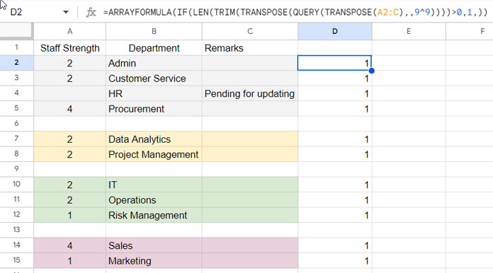
1. Returning 1 or Null Based on Row Emptiness (Value_Expression2)

Formula:

IF(LEN(TRIM(TRANSPOSE(QUERY(TRANSPOSE(data),,9^9))))>0,1,)

Where:

• data = A2:C

Some of you may already be familiar with this formula, previously featured in my tutorial titled Filter Out If the Entire Row Is Blank in Google Sheets.

1. TRANSPOSE(data): The TRANSPOSE function rearranges data from rows to columns.
2. QUERY(TRANSPOSE(data),,9^9): QUERY combines values in each column into the top row.
3. TRANSPOSE(QUERY(TRANSPOSE(data),,9^9)): Transposing it back merges all rows within each row. For a more detailed explanation, please refer to The Flexible Array Formula to Join Columns in Google Sheets.

The TRIM function removes added white spaces, and the LEN function returns the length values in each row. The IF logical test checks if the length is greater than 0, returning 1 for true and blank for false.

The purpose of the above formula is to return 1 in non-blank rows and blank in blank rows.

2. Running Count of Non-Blank Cells in Blank Rows (Value_Expression3)

Formula:

COUNTIFS(empty, "<>"&empty, SEQUENCE(ROWS(data)), "<="&SEQUENCE(ROWS(data)))

Where:

• empty = value_expression2 (refer to column D in the screenshot above)
• data = A2:C

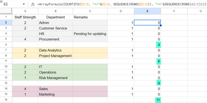
This COUNTIFS formula returns the running count of 1 (column D values) in blank rows.

Syntax of the COUNTIFS Function:

COUNTIFS(criteria_range1, criterion1, [criteria_range2, …], [criterion2, …])

If we only use criteria_range1 and criterion1, the formula will return the cumulative count in each blank row, which will be 11 (the count of total 1 in column D).

This is the key formula to group data separated by blank rows as we have now unique numbers in blank rows. In the next step, we will use this to create unique categories.

3. Replacing 0 with the Value Greater than 0 from the Cell Above (Value_Expression4)

Formula:

In this step, we will use the SCAN lambda function to scan value_expression3 (values in column E above).

SCAN(1, rc, LAMBDA(a, v, IF(v=0, a, v)))

Where:

• rc = value_expression3

Syntax of the SCAN Function:

SCAN(initial_value, array_or_range, lambda)

The function takes two arguments: an accumulator (initial_value) and an array (value_expression3).

The initial value in the accumulator is 1. The formula applies a lambda function to each row and stores the intermediate value in the accumulator. The lambda function returns the value in the accumulator if the row value is 0; otherwise, it returns the value itself.

This process is similar to filling blank cells with the values from the cell above, with the distinction that cells with 0s are filled rather than blank cells.

Take a look at the values in column F. You can observe that we have already grouped data separated by blank rows.

In the next step, which is the formula expression, we will fine-tune the result by removing values in blank rows.

4. Grouping Data Separated by Blank Rows (Formula_Expression)

Formula:

IF(LEN(empty), test, )

Where:

• empty = value_expression2 that identifies blank rows
• test = the result of the SCAN formula.

The formula returns the test result if the row is not blank; otherwise, it returns blank.

This approach allows us to create a category column for grouping and summing data separated by blank rows in Google Sheets.

Now, let’s move on to some practical applications of the created categories.

Grouping and Aggregating Data Separated by Blank Rows

We will use SUMIF and QUERY for the example purpose.

How to get the total staff strength in each group separated by blank rows in our example above?

Insert the formula that categorizes in cell D2. Please scroll up and see the formula just below the title “Formula for Grouping Data Separated by Blank Rows in Google Sheets.” Don’t copy the formulas used in the explanation part.

Then use the below QUERY:

=QUERY(A2:D, "select sum(A) where D is not null group by D label sum(A)''")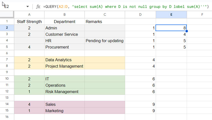

How do we get the total only in the third group?

We can use the same QUERY formula and include OFFSET and LIMIT clauses.

=QUERY(A2:D, "select sum(A) where D is not null group by D limit 1 offset 2 label sum(A)''")

The SUMIF alternative to the above formula is:

=SUMIF(D2:D, INDEX(UNIQUE(TOCOL(D2:D, 1)), 3), A2:A)

Here the TOCOL removes blank rows in the category column, UNIQUE returns the unique values, and INDEX returns the third unique value, which is the criterion in the SUMIF.

How to Replace Category Numbers with Category Texts

In this tutorial, the focus is on generating a category column when dealing with data separated by blank rows that determine the categories. The initial formula generates unique numbers, but if you prefer category texts like “Category A,” “Category B,” and so forth, follow the below workaround.

Using our example:

1. Create categories in column D.
2. In cell G2, enter the following formula to return unique categories (numbers 1, 4, 6, and 9):
   • =UNIQUE(TOCOL(D2:D, 1))
3. In H2:H5, enter the categories “Category A,” “Category B,” “Category C,” and “Category D.”
4. In cell E2, use the following XLOOKUP formula:
   • =ArrayFormula(XLOOKUP(D2:D, G2:G, H2:H, ))

This formula will assign the text categories, providing a clearer representation of your grouped and summed data separated by blank rows in Google Sheets. Check the sample sheet below for reference.

Sample Sheet

Conclusion

Above, I have detailed how to group data separated by blank rows in Google Sheets. Additionally, I have provided 2-3 examples demonstrating how to aggregate the grouped data.

Once you create categories for data separated by blank rows, you can leverage various functions where categories become an integral part.

You can even pivot such data using a Pivot Table or QUERY. If you have any doubts, feel free to ask in the comments below.