Similar to traditional pivot tables, you can pivot multiple columns using the QUERY function in Google Sheets.
This tutorial belongs to the QUERY Pivot & Reporting in Google Sheets hub and covers different QUERY pivot structures using single and multiple GROUP BY and PIVOT fields.
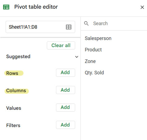
The Pivot Table feature (Insert > Pivot Table) supports multiple fields for grouping under Rows and Columns. Typically, we drag and drop fields into the Rows and Columns sections in the Pivot Table editor and add a field to aggregate under Values.
When using the QUERY function:
- The fields you drag and drop into Rows in a Pivot Table correspond to the fields in the GROUP BY clause.
- The fields you drag and drop into Columns in a Pivot Table correspond to the fields in the PIVOT clause.
Our topic, “Pivot multiple columns using QUERY,” focuses on using multiple fields in the PIVOT clause. Below, I’ve included three examples:
- Single Field in the GROUP BY and PIVOT Clauses
- Multiple Fields in the GROUP BY Clause and a Single Field in the PIVOT Clause
- Single Field in the GROUP BY Clause and Multiple Fields in the PIVOT Clause
(Multiple Columns in Pivot)
Pivot Multiple Columns Using QUERY and Data Requirements
You can pivot multiple columns using the QUERY function, but your data must meet specific requirements. What are they?
The data must have at least three columns: one for grouping (row grouping) and two for pivoting (column grouping). In this case, you can most likely use the COUNT function for aggregation. If your data includes a fourth column with numeric values, you can use it for additional aggregation operations.
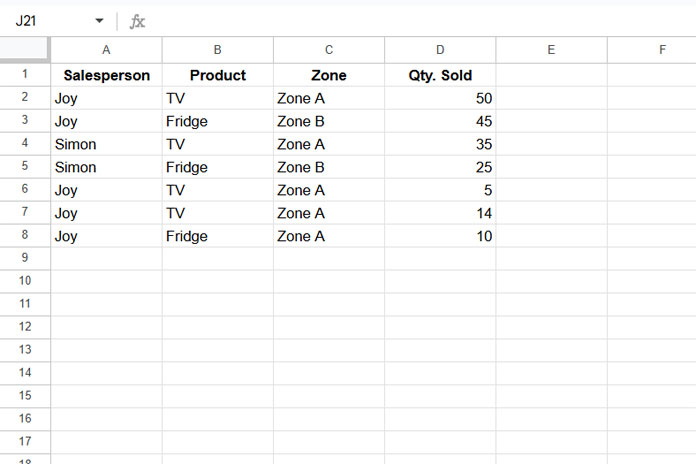
For this tutorial, we’ll use the following sales data. The dataset is well-structured to demonstrate how to pivot multiple columns using the QUERY function.
1. Single Field in the GROUP BY and PIVOT Clauses
Assume you want to create a Pivot Table to show the total sales of products by each salesperson. You can use the following QUERY formula:
=QUERY(A1:D, "SELECT A, SUM(D) WHERE A IS NOT NULL GROUP BY A PIVOT B", 1)Result:
| Salesperson | Fridge | TV |
| Joy | 55 | 69 |
| Simon | 25 | 35 |
Here’s how it works:
- Column A (Salesperson) is used in the GROUP BY clause.
- Column B (Product) is used in the PIVOT clause.
- It’s important to note that any field used in the GROUP BY clause must also be specified in the SELECT clause.
If you were to create this using the built-in Pivot Table feature (Insert > Pivot Table):
- Add Salesperson to Rows.
- Add Product to Columns.
I hope this basic example helps you understand how to pivot multiple columns using the QUERY function later in this tutorial.
2. Multiple Fields in the GROUP BY Clause and a Single Field in the PIVOT Clause
This approach involves using multiple fields in the GROUP BY clause and a single field in the PIVOT clause.
For example, we can group our sample data by Salesperson and Product, and pivot the Zone column. This will provide a summary of each salesperson’s product sales in different regions.
=QUERY(A1:D, "SELECT A, B, SUM(D) WHERE A IS NOT NULL GROUP BY A, B PIVOT C", 1)Result:
| Salesperson | Product | Zone A | Zone B |
| Joy | Fridge | 10 | 45 |
| Joy | TV | 69 | |
| Simon | Fridge | 25 | |
| Simon | TV | 35 |
In this formula:
- Columns A (Salesperson) and B (Product) are used in both the SELECT and GROUP BY clauses.
- Column C (Zone) is used in the PIVOT clause.
If you were to create this using a regular Pivot Table:
- Add Salesperson and Product to Rows.
- Add Zone to Columns.
However, note that the example above is not pivoting multiple columns using the QUERY function. You’ll find that much-awaited example in the section below.
3. Single Field in the GROUP BY Clause and Multiple Fields in the PIVOT Clause (Pivot Multiple Columns Using QUERY)
The following formula groups the Salesperson and pivots the Product and Zone columns:
=QUERY(A1:D, "SELECT A, SUM(D) WHERE A IS NOT NULL GROUP BY A PIVOT B, C", 1)Result:
| Salesperson | Fridge,Zone A | Fridge,Zone B | TV,Zone A |
| Joy | 10 | 45 | 69 |
| Simon | 25 | 35 |
If you were to create this using a regular Pivot Table:
- Add Salesperson to Rows.
- Add Product and Zone to Columns.
When you pivot multiple columns using QUERY or a regular Pivot Table, the result will be wider data compared to the taller data produced by using multiple fields in the GROUP BY clause (multiple columns in Rows in a traditional Pivot Table).
If you compare the output of the last two formulas, you’ll notice that the results are the same, but the arrangement of the data is different.
Ultimately, it’s up to you whether you want to pivot multiple columns or group by multiple columns in QUERY.


Hi Prashanth,
I have the below table.
CUSTOMER NAME | DESCRIPTION | SALE QTY. | TOTAL PRICE | TEAM MEMB | PRODCUT HEAD
FRONT | SP1234 | 6 | 33000 | STAN | SCAN
IMS | AB1234 | 1 | 100000 | BARA | SOFT
FRONT | SP1234 | 1 | 46,422 | NASE | SCAN
ZEN | SP8888 | 1 | 46,422 | STAN | CONSUM
SOFTWARE | AB9876 | 1 | 565488 | NASE | SOFT
FRONT | SP8888 | 10 | 389545 | KINE | SOFT
ABC | XY1234 | 4 | 47,861 | BARA | SERV
IMS | ABA1234 | 1 | 246750 | BARA | SOFT
How to get the below output using Query pivot function?
TEAM MEMB | CUSTOMER NAME | DESCRIPTION | SALE QTY | SCAN | SOFT | CONSUM | SERV
STAN | FRONT | SP1234 | 7 | 79422
BARA | IMS | AB1234 | 2 | 346750
Rgds
Hari
Hi, Hari,
As far as I know, that’s not possible or easy to create with a Query Pivot Table. But I have a very clean formula based on SORTN and SUMIF array combination.
I’ll consider writing a tutorial based on your above input. In the meantime, please give me access to your sheet which I’ve already sent.
Note: In your sample, I think the team member corresponding to SP1234 is “STAN” in row # 2 and 4.
Hi, Hari,
From your sheet, I could realize that the offered SUMIF and SORTN combo is not practical. So to solve the problem, I have used two Query formulas in the nested form.
One Query uses the Pivot clause whereas the other doesn’t.
For other readers, the above data range is in A2:F10. For that range, I’ve used the following nested Query to summarize the data.
={query(A2:F10,"Select E,A,B, sum(D) group by E,A,B pivot F",1),query(A2:F10,"Select sum(C) group by E,A,B label sum(C) 'SALE QTY' ",1)}Best,
GROUP BY and PIVOT is not working at the same time. It shows an error to me. How can I solve the problem?
Hi, Tham,
There is no such issue with Query! Are you using the Query clauses in the correct order?
Related: What is the Correct Clause Order in Google Sheets Query?
Without seeing the data and error, I won’t be able to comment further. You can consider sharing a screenshot showing error value or a sample of your sheet which won’t be published.