This post explains how to use OR logic in COUNTIFS across either column in Google Sheets. The best way to solve this is by using QUERY.

If you wish to use COUNTIFS, you may need to use it unconventionally. Here, I’ll explain that and include the QUERY solution. Before that, here is the scenario to understand the problem.

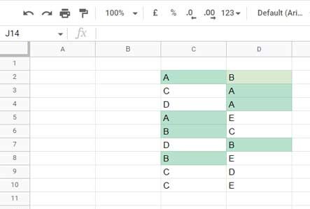
Assume five players compete in a tournament, and their fictional names are A, B, C, D, and E.

In my sample data, C2:D contains player names where each player in C2:C will compete with the corresponding player in D2:D by the end of the tournament.

I want to find the total matches played by players A and B by counting rows where either C2:C or D2:D contains A or B—in other words, applying OR logic in COUNTIFS across either column.

Here is how to find it.

OR Logic in COUNTIFS Across Either Column

We can’t apply the OR function in an array without using resource-hungry Lambda helper functions. So we will use the + operator.

The following formula will return either 0, 1, or 2 depending on the presence of A or B in cells C2 and D2:

=(C2="A")+(C2="B")+(D2="A")+(D2="B")

For example, with the sample data, the output will be:

=TRUE+FALSE+FALSE+TRUE

Where TRUE = 1 and FALSE = 0, so the result will be 2. This means if the value is greater than 0, then either A or B is present.

We need to apply this to the range C2:C and D2:D. So we require the ARRAYFORMULA:

=ArrayFormula((C2:C="A")+(C2:C="B")+(D2:D="A")+(D2:D="B"))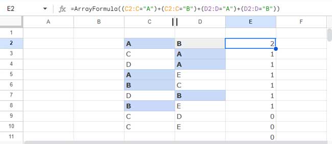

In COUNTIFS, use this as the criteria range and “>0” as the criterion:

=COUNTIFS(ArrayFormula((C2:C="A")+(C2:C="B")+(D2:D="A")+(D2:D="B")), ">0")

The formula will return 7, indicating that players A and B played 7 matches.

This is an example of applying OR logic in COUNTIFS across either column in Google Sheets.

QUERY Alternative

We can use the QUERY function as an alternative to replace OR in COUNTIFS across either column in Google Sheets.

The QUERY function applies an SQL-like query to the range C2:D.

Formula:

=QUERY(C2:D, "SELECT COUNT(C) WHERE C MATCHES 'A|B' OR D MATCHES 'A|B' LABEL COUNT(C)'' ")

This formula uses the QUERY function to count the number of rows in the range C2:D where either column C or column D matches ‘A’ or ‘B’.

It uses the MATCHES regular expression match to filter rows where columns C or D match either ‘A’ or ‘B’.

The LABEL clause in the formula removes the default label from the result.

Resources

• COUNTIFS with Multiple Criteria in Same Range in Google Sheets
• Google Sheets: COUNTIFS with Not Equal to in Infinite Ranges
• COUNTIFS in a Time Range in Google Sheets [Date and Time Column]
• Not Blank as a Condition in COUNTIFS in Google Sheets
• COUNTIF | COUNTIFS Excluding Hidden Rows in Google Sheets
• How To Use COUNTIF or COUNTIFS In Merged Cells In Google Sheets
• Varying Array Sizes in COUNTIFS in Google Sheets
• OR Logic in Multiple Columns with COUNTIFS in Google Sheets
• COUNTIFS with ISBETWEEN in Google Sheets
• Counting XLOOKUP Results with COUNTIFS in Excel and Google Sheets