Using the combination of IF, AND, and OR functions directly in an array in Google Sheets isn’t feasible with the standard approach. However, there are alternative options available.
One involves utilizing operators such as multiplication (*) and addition (+) to replace AND and OR, while the other is to use the MAP lambda function.
I’m discussing combining the IF, AND, and OR logical functions within an array.
I’ve already created tutorials in two distinct posts on utilizing the OR and AND logical functions separately within an array. You can find them under the “Resources” section at the end of this tutorial.
Understanding the Constraints of IF, AND, and OR in Array Utilization
In the following examples, column A contains the names of employees, column B lists their departments, and column C specifies their allocated projects.
To evaluate each record and return “Selected” if the department in column B is electrical and the project in column C is either Project 1 or Project 2, a formula combining IF, AND, and OR logical functions is used, as shown in the screenshot below.
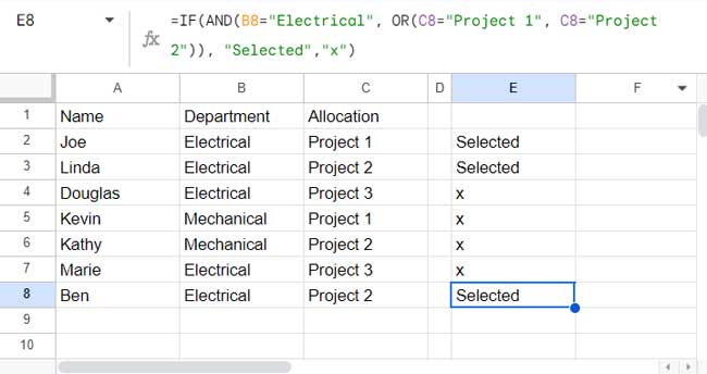
In cell E2, the following formula is applied:
=IF(AND(B2="Electrical", OR(C2="Project 1", C2="Project 2")), "Selected","x")This formula is then dragged down from cell E2 to apply it to each row.
However, the goal is to have a single formula in cell E2 that expands results down.
Simply replacing B2 and C2 with B2:B and C2:C and entering the formula as an array formula won’t yield the desired outcome.
Here are two alternative approaches to utilizing IF, AND, and OR with arrays in Google Sheets.
Two Methods for Utilizing IF, AND, and OR with Arrays
Below, you will find how to use IF, AND, and OR in an array by using multiplication and addition operators with IF in Google Sheets. Additionally, we will see an example using LAMBDA.
Using Multiplication and Addition Operators with IF
I suggest mastering this simple technique, as it proves useful in functions such as SUMPRODUCT, SUMIF, COUNTIF, etc., where conditions are utilized.
Here’s the logic:
When evaluating a cell value like =A2="Apple" in a sheet, it returns the Boolean value TRUE (1) or FALSE (0).
=(A2="Apple")*(B2="Orange") will return 1 if both tests evaluate to TRUE; otherwise, it returns 0. This is equivalent to =AND(A2="Apple", B2="Orange").
=(A2="Apple")+(B2="Orange") will return 2 if both tests evaluate to TRUE, 0 if both tests evaluate to FALSE, and 1 if either of the tests evaluates to TRUE. This is equivalent to =OR(A2="Apple", B2="Orange").
This is the logic behind using multiplication and addition operators instead of the AND or OR logical functions.
So we can replace =AND(B2="Electrical", OR(C2="Project 1", C2="Project 2")) with =(B2="Electrical")*((C2="Project 1")+(C2="Project 2")).
Therefore, we can replace the earlier non-array formula in cell E2 with the following formula:
=IF((B2="Electrical")*((C2="Project 1")+(C2="Project 2")), "Selected", "x")Unlike the previous formula, this will work as an array formula:
=ArrayFormula(IF((B2:B8="Electrical")*((C2:C8="Project 1")+(C2:C8="Project 2")), "Selected", "x"))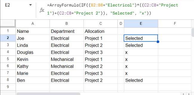
Using MAP Lambda Function
The MAP function in Google Sheets allows you to apply a custom LAMBDA function to corresponding elements in one or more arrays.
Let’s see how to convert our non-array IF, AND, and OR combination to a custom lambda function to use in MAP.
Non-Array:
=IF(AND(B2="Electrical", OR(C2="Project 1", C2="Project 2")), "Selected", "x")Custom Lambda Function:
When converting the above formula (or any formula) to a custom lambda function, you can use meaningful names to assign to the cell references.
=LAMBDA(department, project, IF(AND(department="Electrical", OR(project="Project 1", project="Project 2")), "Selected", "x")This custom function follows the syntax LAMBDA([name, …], formula_expression), where:
name1: departmentname2: projectformula_expression:IF(AND(department="Electrical", OR(project="Project 1", project="Project 2")), "Selected", "x")
Now let’s specify the arrays B2:B8 and C2:C8 within MAP to return an array output.
=MAP(B2:B8, C2:C8, LAMBDA(department, project, IF(AND(department="Electrical", OR(project="Project 1", project="Project 2")), "Selected", "x")))Syntax:
MAP(array1, [array2, …], lambda)Where:
array1: B2:B8array2: C2:C8lambda:LAMBDA(department, project, IF(AND(department="Electrical", OR(project="Project 1", project="Project 2")), "Selected", "x"))
Resources
- How to Use AND Logical in Array in Google Sheets
- Using OR Logical Function to Return Expanded Results in Google Sheets
- Combined Use of IF, AND, and OR Logical Functions in Google Sheets
- AND, OR, or NOT in Conditional Formatting in Google Sheets
- Logical AND, OR Use in SEARCH Function in Google Sheets
- How to Correctly Use AND and OR Functions with IFS in Google Sheets


Hi, Les Mint,
Thanks for your valuable feedback.
Happy New Year 2023 – may you have good health, experiences, and company.
Hi Prashanth,
Any advice for getting this ARRAY to work? The formula works, but the ARRAY cannot be used with AND/OR as you’ve described.
=ARRAYFORMULA(IF(OR(ISBLANK(B2),ISBLANK(C2),ISBLANK(E2),ISBLANK(G2),ISBLANK(H2)),0,1))
Thanks!
Hi, Benny Harris,
This formula may do the trick.
=ArrayFormula(if(len(B2:B10)*len(C2:C10)*len(E2:E10)*len(G2:G10)*len(H2:H10)>0,1,0))
You can also use a MAP lambda formula.
=map(B2:B10,C2:C10,E2:E10,G2:G10,H2:H10,lambda(b,c,e,g,h,if(or(isblank(b),isblank(c),isblank(e),isblank(g),isblank(h)),0,1)))
I’ve updated my tutorial to include a MAP solution w.r.t. the example there.
Hi Prashanth!
I’m hoping you can help.
I have a Google Sheet with multiple tabs.
If the ID number in column D of one tab matches an ID number in column E of another tab, I want a YES or TRUE or anything in column G of the first tab.
How do I do this?
Hi, Allison B,
Assume the tabs in question are Sheet1 and Sheet2.
Empty Sheet1 column G and enter the following IF and MATCH combo in G1.
=ArrayFormula(ifna(if(match(D:D,Sheet2!E:E,0),"YES",)))I know I cannot use AND() in an Array Formula, but if I wanted to turn the formula below into an Array, any tips on how to do that?
=(IF(AND(J:J="- Not Field Trained via CFT -",I:I="- Currently not Peer Supported -"),"No","Yes"))
Hi, Wyatt,
You can try this formula.
=ArrayFormula(if(len(J:J&I:I),if((J:J="- Not Field Trained via CFT -")*(I:I="- Currently not Peer Supported -"),"No","Yes"),))
That worked!!! Thank you! What is LEN, if you do not mind me asking?
Hi, Wyatt,
To test whether the cell has any character. The LEN returns the length of the string in that cell.
I feel like this is the exact place I need to find out how to turn this IF AND into an ARRAY, but I keep coming up short.
Here is the formula that I want to convert:
=IF(AND(J2>0,U20)*(U2:U0,""))I’d appreciate any help!
Hi, Chris,
I’m not clear. Can you please leave the URL of your example sheet, if any, below in your reply?
Hello Prashanth,
Here’s a screenshot of my google sheet derived from a google form: — link removed by admin —
I need to auto-populate the ‘Remarks” column with either a “Pass” or “Fail” value based on the answers on all Q columns.
I tried arrayformula for IF, AND, OR. But as you mentioned, they don’t work.
Please enlighten me on how? 🙂
Thanks!
Hi, Paul,
Thanks for the screenshot.
I have noted the values/answers in columns B, C, D, E, and F.
In column G, you want the Pass/Fail in each row.
But what are the conditions for Pass or Fail?
Thank you for the reply Prashanth.
Answers to questions should be satisfied.
Example: Q1=Yes, Q2=NSW, Q3>=59, Q4=Yes, Q5=No/Unsure.
If all is true, remarks will be “Passed.”
Thanks,
Paul
Hi, Paul,
Thanks for your explanation.
Empty the range G2:G. Then, please insert the following array formula in G2.
=ArrayFormula(if(B2:B="",,if((B2:B="Yes")*(C2:C="NSW")*(D2:D=59)*(E2:E="Yes")*
((F2:F="No")+(F2:F="No/Unsure")),"Passed","Failed")
))
Brilliant! Thank you.
Prashanth, that worked. Thank you.
Hi Scott,
The simple formula I had was working fine. But now we have added another factor to it.
I am currently using
=Countifs($i$3:$I$154, L10, $g$3:$g$154, ">=500")I cannot figure out how to manipulate it to pump it against column J to take only = “Loss.”
Any help would be greatly appreciated.
Hi, Les Sullivan,
Try this first.
=Countifs(I3:I154, L10, G3:G154, ">=500",J3:J154,"Loss")If not working as expected, please share the URL of the sheet in problem or a sheet with sample data below “Reply to this comment”.
I will keep your “reply” unpublished.
Hello,
I’m trying to create an if/and formula. Based on the criteria select, I want it to display a table. Not sure how to make that work with an array formula.
Hi, Scott Miller,
Can you share an example sheet below?
N.B. – I won’t publish it.
Hi Prashanth,
Thanks for this site, it has been so incredibly helpful, my Sheets skills have improved dramatically thanks to your very clear and concise explanations. Things that other sites have suggested very complicated solutions to, or just said are not possible, you have offered a simple solution.
Really appreciate it.
Hi, Steve,
Thanks for your feedback!
This guide came in clutch. Thanks!!
Hi Prashanth,
I have the day divided into 2 sections “Turno 1 and “Turno 2” depending on the time printed on the ticket at the moment the order was made.
So Im trying the formula to return in witch one is it, 1 or 2 I have it l like this:
=arrayformula(if(and(AD2:AD>time(11,0,0),AD2:ADtime(17,0,0)),"Turno 2")))Based on what I’ve found on google I’ve modified a couple of times but nothing seems to work it keeps coming wrong or with an error.
Do you think there’s a way to make it work? or should I give up?
Thanks!
Hi, Viri,
Please clarify the time period.
Like;
11:00:00 to 17:00:00 – Turno 2
17:00:00 to 22:00:00 – Turno 1
So that I can write the formula. You might want to use multiple IF instead of AND within IF.
I would like to create an ArrayFormula which adds up hours based on words in a cell for the row, not the column, but I do want it to do the same function for the entire sheet.
So I would like it to look at all the rows starting in column
F10 - AG10for the wordsMOECSUpload orCofCand then add the hours the person would receive located in row 6 of the same column those words are in. I can share my sheet if you need to see it.Hi, Erika Rupert,
The hours are in row # 6 (F6:AG6).
In row # 10 (AH10), you want to sum the above hours if the values in row # 10 (F10:AG10) are
MOESorCofC.The same you want to repeat in row # 11, row # 12, and so on.
I’ve two options. One is a drag-drop formula and the other is an array formula. But first, you must format your row # 6. Instead of 3 Hrs, just enter 3, so that we can sum.
Drag-drop Formula (Formula should be keyed in cell AH10 and then drag-down (copy-paste down):
I think, here instead of using IF, AND, OR logical functions in array use, we can use FILTER and REGEXMATCH combo.
=sum(ifna(filter($F$6:$AG$6,regexmatch(F10:AG10,"MOECS|CofC"))))Self Expanding Formula (Formula should only be keyed in cell AH10 (AH11:AH should be empty):
=ArrayFormula(mmult(if((F10:AG343="MOECS")+(F10:AG343="CofC")=1,F6:AG6,0),transpose(column(F6:AG6)^0)))In this formula, the MMULT matrix1 is actually a combination of IF, OR logical in array use.
Hi there,
I just want to do an array on only IF/ AND.
My formula looks like this
=ArrayFormula(IF(AND(AK$2:AK=Key!C$7, AL2:AL="No",AM2:AM="Easy"),Key!F$37))How would I make it work, please?
E
Hi, Evan,
The AND logical function won’t work with the ArrayFormula as above. Here is the correct approach.
=ArrayFormula(IF((AK$2:AK=Key!C$7)*(AL2:AL="No")*(AM2:AM="Easy")>0,Key!F$37,))I have written this formula without seeing your data. So if not working you can share a screenshot of your data.
Best,
Hi,
I want to find the cash spent by a person. I’m not sure what formula I need to use?
Can you please help with that?
Requirement:
Column A, Column B
Name1, 100
Name2, 300
Name1, 500
I want to find the total amount spent by a person (say Name 1)… How can I calculate it?
Hi, Sri Ram,
It has nothing to do with IF, AND, OR functions or combination. Still, here are my solutions.
There are several functions that you can use to solve your said problem. To name a few, SUMIF, QUERY, and FILTER.
Formula based on SUMIF:
=sumif(A1:A,"Name 1",B1:B)Based on Filter:
=sum(filter(B1:B,A1:A="Name 1"))The last formula based on Query:
=query(A1:B,"Select Sum(B) where A='Name 1'")Pick the one that you may find simple to understand. Actually, all these functions, except Query, are easy to learn. Please check my Google Sheets Function Guide.
Best,
Thanx for the post.
Now, I know where to look if stuck in Google Sheet.