This post explains how to use AND, OR in the SEARCH function in Google Sheets.
Normally in most of the logical formulas, we use the plus (+) sign for the OR use and an asterisk (*) for the AND use. But the fact here is that we will use none of them with the SEARCH function.
Interesting, right?
First, you may go through some examples of the AND, OR functions in standalone use. Understanding them will clear your doubts about why I am not using them with the SEARCH function.
The OR returns TRUE if any of the arguments are TRUE in a logical test.
=or(F4="apple",F4="orange")This we can replace with the below formula which would return a value greater than zero if any of the arguments are logically TRUE.
=(F4="apple")+(F4="orange")The AND returns TRUE if all of the arguments are TRUE in a logical test.
=and(F4="apple",F5="orange")The same formula, we can rewrite using the asterisk operator as below.
=(F4="apple")*(F5="orange")If the result is 1, that means all of the arguments are TRUE.
Here, in the AND use, the formula tests the values from two different cells, not from a single cell.
The SEARCH function is for partial matches.
So in AND use in the SEARCH in Google Sheets, we can refer to the same cell twice for the logical test. I mean, both the strings “apple” and “orange” can be checked in cell F4 itself.
In AND, OR Use in SEARCH Function in Google Sheets, we won’t use the AND, OR functions or its alternative operators! I’ll explain the same with a few examples below.
AND, OR Use in SEARCH Function (Alternatives)
Here I am going to give more importance to the OR use in SEARCH than AND use in SEARCH. Once you have gone through the below examples, you will understand why it is so.
OR Use in the SEARCH Function
Example 1
Assume cell C2 contains the word “train timing”
I want to check whether cell C2 contains any of the text train, bus, flight, tram, or metro.
If any of the above texts are present in cell C2, return “Transportation” else “Unknown Mode of Transportation”!
=if(
     sum(
        iferror(
           ArrayFormula(
              search({"Train";"Flight";"Bus";"Tram";"Metro"},C2)
           )
        )
     )>0,
     "Transportation","Unknown Mode of Transportation"
)
I will give you one more example, and in that, I’ll try to explain the formula in detail.
Example 2 (Step by Step Approach)
You are learning the OR part in the AND, OR use in the SEARCH function in Google Sheets.
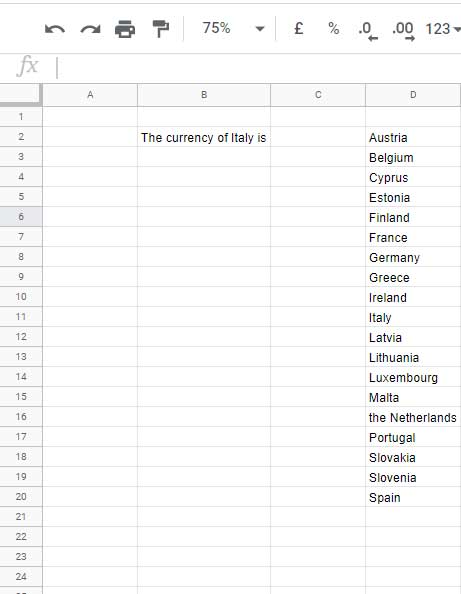
In cell B2, I have a country name within a sentence. I want to test whether it is a country that uses the EURO currency.
The value in cell B2 is as follows – The currency of Italy is.
We should know whether “Italy” matches in the list of member countries who are using the EURO currency.
So make a list of member countries who are using the EURO currency as a list in D2:D.

Here the text to search is the string in cell B2.
Syntax:
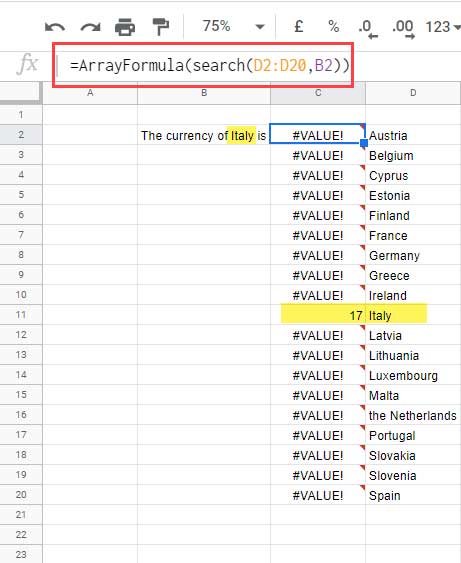
SEARCH(search_for, text_to_search, [starting_at])We will search the 19 countries (the countries who are using the EURO currency) in the range D2:D20 as below.
=ArrayFormula(
     search(D2:D20,B2)
)
Note:- We can specify/hardcode the range D2:D20 as below too.
{"Austria";"Belgium";"Cyprus";"Estonia";"Finland";"France";"Germany";"Greece";"Ireland";"Italy";"Latvia";"Lithuania";"Luxembourg";"Malta";"the Netherlands";"Portugal";"Slovakia";"Slovenia";"Spain"}I have used the ArrayFormula function because the search_for is an array.
The SEARCH function returns the position of the serch_for (D2:D20) in text_to_search (B2) by counting the characters in the cell B2.
If the total of the above formula result is greater than zero, then return “Euro”, else “Unknown”.
Before summing the above result, we should eliminate the #VALUE! errors. Then only the SUM would work. We can use IFERROR for that.
=if(
     sum(
        iferror(
           ArrayFormula(
              search(D2:D20,B2)
           )
        )
     )>0,
     "Euro","Unknown"
)
Change the text in cell B2 to The currency of Japan is. The formula would return “Unknown”.
You have learned the OR use in SEARCH. Now in our AND, OR Use in SEARCH Function in Google Sheets, the next part is the AND use.
AND Use in the SEARCH Function
In AND use in the SEARCH function, we want to check the presence of multiple keywords in the text_to_search part of the formula.
For example, the value in cell D1 is “diesel injection pump”. I want to test the presence of the words “diesel” and “pump” in this string.
First we will search “diesel” in D1. The formula for the same is;
=ArrayFormula(
     IFERROR(
        search("diesel",D2)
     )
)
Now let’s search “pump” using the following SEARCH formula.
=ArrayFormula(
     IFERROR(
        search("pump",D2)
     )
)
If the count of both the result is 2, that means both the words are present.
=count(
     ArrayFormula(IFERROR(search("diesel",D2))),
     ArrayFormula(IFERROR(search("pump",D2)))
)
Note:-
Most of the time, in an array formula similar to the one above, no need to depend on more than one ArrayFormula function.
You can remove the inner Array Formulas and corresponding open/clause brackets and then wrap the entire formula with a single ArrayFormula.
The above are examples of the use of logical AND, OR in SEARCH function in Google Sheets.
Related Resources
- Multiple Search Strings in a Single SEARCH Formula in Google Sheets.
- Google Sheets FIND Function and Its Difference with SEARCH Formula.
- How to Use MID, SEARCH Functions in Google Sheets [Text Functions].
- Combined Use of IF, AND, OR Logical Functions in Google Doc Spreadsheet.
- How to Use IF, AND, OR in Array in Google Sheets.
- How to Correctly Use AND, OR Functions with IFS in Google Sheets.
- AND, OR, or NOT in Conditional Formatting in Google Sheets.
- AND, OR in Multiple Criteria DSUM in Google Sheets (Within Formula).
- How to Use And, Or, and Not in Google Sheets Query.


