Using DSUM with multiple criteria is easy when referencing criteria from cell values. However, when using hardcoded criteria, you must correctly structure the criteria array within the formula.
Understanding AND and OR Logic in DSUM
This isn’t about using the AND and OR functions inside DSUM. Instead, it’s about handling multiple criteria in the same column or across different columns.
- OR Logic: Multiple criteria in the same column
- AND Logic: One criterion per different columns
- AND + OR Logic: A combination of both
Let’s break it down with simple examples below.
Sample Data
We’ll use the following dataset where students’ marks in different subjects are recorded across terms:
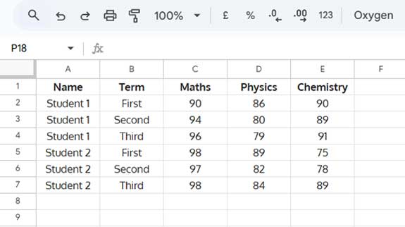
To apply AND and OR logic in DSUM with multiple criteria, we will filter based on Name and Term.
DSUM with a Single Criterion in Google Sheets
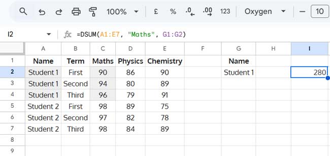
Suppose you want to sum the Maths marks for Student 1.
Criterion as Cell Reference
- Enter
"Student 1"in cellG2, below the label"Name"inG1. - Use this formula:
=DSUM(A1:E7, "Maths", G1:G2)
Explanation
- Database:
A1:E7(data range) - Field:
"Maths"(the column to sum) - Criteria:
G1:G2(filters the data)
If you leave G2 empty, the formula returns the sum of all students.
Criterion within Formula (Hardcoded)
Instead of using cell references, you can hardcode the criteria using VSTACK:
=DSUM(A1:E7, "Maths", VSTACK("Name", "Student 1"))VSTACK creates a vertical array, replicating the criteria range within the formula.
DSUM with Multiple Criteria in Google Sheets
OR Condition in Multiple Criteria DSUM
When using multiple conditions in the same column, DSUM applies OR logic automatically.
Criteria as Cell Reference
- Enter student names below
"Name"inG1, e.g.,"Student 1","Student 2","Student 3". - Use this formula:
=DSUM(A1:E7, "Maths", G1:G4)
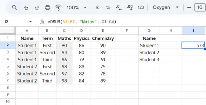
This formula sums Maths marks if the Name is “Student 1” OR “Student 2” OR “Student 3”.
Criteria within Formula (Hardcoded)
=DSUM(A1:E7, "Maths", VSTACK("Name", "Student 1", "Student 2", "Student 3"))AND Condition in Multiple Criteria DSUM
If all conditions are met, DSUM applies AND logic.
Criteria as Cell Reference
- Enter “Student 1” in G2 and “Second” in H2. Assume the relevant field labels are present in G1:H1.
- Use this formula:
=DSUM(A1:E7, "Maths", G1:H2)
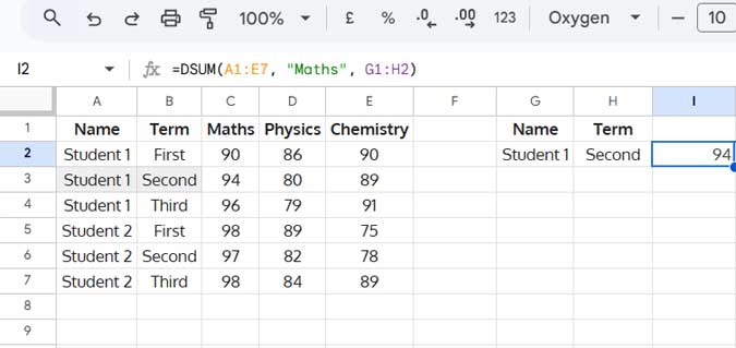
This sums Maths marks only if Name = “Student 1” AND Term = “Second”.
Criteria within Formula (Hardcoded)
=DSUM(A1:E7, "Maths", HSTACK(VSTACK("Name", "Student 1"), VSTACK("Term", "Second")))Explanation
VSTACK("Name", "Student 1"): Creates a column for Name criteriaVSTACK("Term", "Second"): Creates a column for Term criteriaHSTACK(...): Combines them into a 2D array for DSUM
AND + OR Condition in Multiple Criteria DSUM
Now, let’s mix AND and OR logic.
Example: Sum Maths Marks for Student 1 in Term 1 OR Term 2
| Name | Term |
| Student 1 | First |
| Student 1 | Second |
If this table is in G1:H3, the formula is:
=DSUM(A1:E7, "Maths", G1:H3)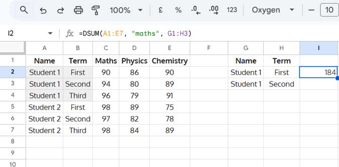
Criteria within Formula (Hardcoded)
=DSUM(A1:E7, "Maths", HSTACK(VSTACK("Name", "Student 1", "Student 1"), VSTACK("Term", "First", "Second")))This sums Maths marks where Name = “Student 1” AND Term = (“First” OR “Second”).
Exact Match in Multiple Criteria DSUM
By default, DSUM performs partial matches. "Student 1" would match "Student 11".
To enforce exact match, use =Student 1 instead of Student 1.
Example:
=DSUM(A1:E7, "Maths", VSTACK("Name", "=Student 1"))Note: When entering this criterion in a cell, you may encounter issues. To avoid this, start with an apostrophe ('), like '=Student 1.
Final Thoughts
You’ve now learned how to use AND and OR in multiple criteria DSUM in Google Sheets. Whether you need to sum values based on a single condition, multiple OR conditions, AND conditions, or a mix of both, DSUM provides a flexible solution.
Key Takeaways
- OR condition: Multiple values in the same column
- AND condition: One value per different column
- AND + OR condition: Multiple criteria in multiple columns
- Hardcoded criteria: Use
VSTACKandHSTACK
For structured filtering and summing, DSUM is an efficient alternative to SUMIFS.


=DSUM(A1:I31,"Item_Value",{"Who","him";"Asset_Debt","Asset"})The above formula does NOT sum up ‘Item_Value’ for all records having ‘him’ in the ‘Who’ field #AND# having ‘Asset’ in the ‘Asset_Debt’ field.
Hi, Mike H,
Your criteria use is wrong.
As per my Sheet’s Locale, which is the UK, it must be as below.
transpose({"Who","him";"Asset_Debt","Asset"})If you see error even after making the above change, then see this Locale setting guide – How to Change a Non-Regional Google Sheets Formula.
If you let me know your sheets’ ‘Locale’, then I may be able to tune the formula for you.