Are you seeing the “Array arguments to COUNTIFS are of different sizes” error in Google Sheets? This error occurs when you use varying array sizes in a COUNTIFS formula, as the function doesn’t support arrays of different sizes.
This issue typically arises when the columns specified in criteria_range1 and criteria_range2 have mismatched sizes.
It’s important to understand the function syntax:
Syntax: COUNTIFS(criteria_range1, criterion1, [criteria_range2, …], [criterion2, …])
When specifying multiple criteria ranges, the dimensions of the criteria ranges must be the same.
This means the number of rows and columns must match across all specified criteria ranges or arrays. Let’s look at an example to illustrate this:
=COUNTIFS(A2:D10, "Apple", E2:E10, "Yes")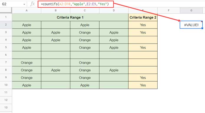
In this example, I want to count the occurrences of “Apple” in the multi-column range A2:D10 where the corresponding value in E2:E10 equals “Yes.” However, this returns a #VALUE! error.
In this formula, four arguments are in use:
criteria_range1– A2:D10criterion1– “Apple”criteria_range2– E2:E10criterion2– “Yes”
As you can see, the two array arguments (criteria_range1 and criteria_range2) provided to COUNTIFS have different sizes.
The first array (criteria_range1) has four columns, while the second array (criteria_range2) has only one column.
I have three workaround formulas for you to try when you encounter the #VALUE! error due to varying array sizes in COUNTIFS, as described above.
Option 1: Expanding Criteria Range Dimensions
In our example, criteria_range1 (A2:D10) contains 4 columns, while criteria_range2 (E2:E10) contains 1 column.
To match the number of columns in criteria_range1, you need to expand criteria_range2 to 4 columns. You can achieve this by repeating the column multiple times using the SUBSTITUTE function as follows:
=ArrayFormula(SUBSTITUTE(E2:E10, "", SEQUENCE(1, 4)))This formula repeats the values in E2:E10 across 4 columns (you can adjust the number of repetitions by changing the 4 in the SEQUENCE function to the desired number).
Use this adjusted range as criteria_range2 in your COUNTIFS formula:
=COUNTIFS(A2:D10, "Apple", ArrayFormula(SUBSTITUTE(E2:E10, "", SEQUENCE(1, 4))), "Yes")Matching the criteria range dimensions is one way to handle varying array sizes in COUNTIFS. However, there are several alternative solutions. Below, you’ll find two of the best alternatives.
Option 2: Filtering a Multi-Column Range
You can achieve the desired result without matching varying array sizes in COUNTIFS as described above.
The goal is to count “Apple” in A2:D10 where E2:E10 is “Yes.” To do this, we’ll filter A2:D10 based on the condition in E2:E10, which allows us to avoid using criteria_range2.
Use the following formula:
=COUNTIFS(FILTER(A2:D10, E2:E10="Yes"), "Apple")The FILTER function filters A2:D10 to include only the rows where E2:E10 equals “Yes.” Then, COUNTIFS is used to count the occurrences of “Apple” within the filtered range.
Option 3: Using an IF Logical Test
This approach is similar to Option 2. Instead of using FILTER, we will eliminate criteria_range2 using an IF logical test:
=COUNTIFS(ArrayFormula(IF(E2:E10="Yes", A2:D10,)), "Apple")The formula ArrayFormula(IF(E2:E10 = "Yes", A2:D10,)) returns the values from A2:D10 where E2:E10 is equal to “Yes”; otherwise, it returns blank.
Within this multi-column range, COUNTIFS is used to count occurrences of “Apple.”
Handling Varying Array Sizes in COUNTIFS: Choosing the Best Option
Out of the three formulas, I would recommend Option 2. Option 1 may impact performance with large datasets. Option 2 is preferable to Option 3 as well, in terms of performance, since it operates on a smaller, filtered dataset rather than the entire range.
Resources
- How to Count If Not Blank in Google Sheets [Tips and Tricks]
- COUNTIFS with Multiple Criteria in the Same Range in Google Sheets
- Google Sheets: COUNTIFS with Not Equal to in Infinite Ranges
- COUNTIFS in a Time Range in Google Sheets [Date and Time Column]
- COUNTIF | COUNTIFS Excluding Hidden Rows in Google Sheets
- How To Use COUNTIF or COUNTIFS In Merged Cells In Google Sheets
- Using ‘Not Blank’ as a Condition in COUNTIFS in Google Sheets
- OR Logic in Multiple Columns with COUNTIFS in Google Sheets
- OR Logic in COUNTIFS Across Either Column in Google Sheets
- COUNTIFS with ISBETWEEN in Google Sheets
- Counting XLOOKUP Results with COUNTIFS in Excel and Google Sheets


