In this post — Sum of matrix rows or columns in Google Sheets — let’s look at how to get a total row or column using the SUMIF function.
You might’ve seen total rows or columns in pivot tables. But what if you’re working in a normal table or array? We can create similar total rows or columns using SUMIF, without needing to build a pivot.
Usually, to calculate the sum of matrix rows (a total column on the right of a range) or matrix columns (a total row at the bottom), we use the BYROW or BYCOL function. Earlier, we relied on MMULT, DSUM, or QUERY. I’ve already explained part of that in my post on How to Sum Each Row in Google Sheets.
But we can do the same using a clever SUMIF trick too.
You might ask — is this really necessary? Maybe not, but it’s a neat trick to know!
So let’s go through how to get the sum of matrix rows or columns using SUMIF in Google Sheets.
Can We Really Use SUMIF to Get Row or Column Totals?
You might know that the main purpose of SUMIF is to do a conditional sum.
But here, we don’t have any “conditions” — just a matrix and a goal: total up each row or column.
So how do we make that work?
SUMIF Logic for Total Rows and Columns in Google Sheets
Let’s say you have a matrix in range C3:F7.
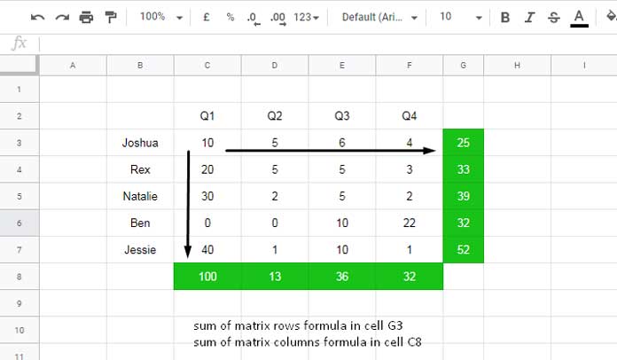
Our goal is to:
- Get row totals in
G3:G7 - Get column totals in
C8:F8
This is similar to what a pivot table might do — just manually.
In an earlier tutorial, I showed how to get totals from multiple columns using SUMIF by duplicating the range. We’re doing something similar here — except this time, we’re not using real “criteria” or a “range.”
We’re building virtual ones using ROW and COLUMN.
Let me explain.
Sum of Matrix Rows Using SUMIF in Google Sheets
We want the row totals from the matrix C3:F7, and we want to display them in G3:G7.
This matrix has 5 rows and 4 columns.
Step 1: Create a virtual “range” — a matrix of row numbers
=ArrayFormula(IF(COLUMN(C3:F3), ROW(C3:F7)))This gives us a grid filled with the corresponding row numbers — same shape as our matrix.
| 3 | 3 | 3 | 3 |
| 4 | 4 | 4 | 4 |
| 5 | 5 | 5 | 5 |
| 6 | 6 | 6 | 6 |
| 7 | 7 | 7 | 7 |
Step 2: Set the criteria — actual row numbers (one column only)
=ArrayFormula(ROW(C3:C7))3
4
5
6
7
Step 3: Final formula to get row totals (in G3)
=ArrayFormula(SUMIF(IF(COLUMN(C3:F3), ROW(C3:F7)), ROW(C3:C7), C3:F7))This gives you the sum of each row — a total column on the right of your matrix.
Sum of Matrix Columns Using SUMIF in Google Sheets
Now let’s get the column totals. We want the sum of elements in each column of C3:F7, and we’ll output that in C8:F8.
This matrix spans columns C to F and has 5 rows.
Step 1: Create a virtual “range” — a matrix of column numbers
=ArrayFormula(IF(ROW(C3:C7), COLUMN(C3:F7)))This returns a grid where each cell holds the column number — again, matching the matrix shape.
| 3 | 4 | 5 | 6 |
| 3 | 4 | 5 | 6 |
| 3 | 4 | 5 | 6 |
| 3 | 4 | 5 | 6 |
| 3 | 4 | 5 | 6 |
Step 2: Set the criteria — actual column numbers (one row)
=ArrayFormula(COLUMN(C3:F3))3 4 5 6
Step 3: Final formula to get column totals (in C8)
=ArrayFormula(SUMIF(IF(ROW(C3:C7), COLUMN(C3:F7)), COLUMN(C3:F3), C3:F7))This returns the sum of each column — like a pivot table’s total row.
Conclusion
We usually don’t think of SUMIF as a tool for matrix operations — but with a little creativity, it can handle sum of matrix rows or columns quite well.
If you’re already comfortable with SUMIF, this is a great way to reuse that knowledge in new ways. No need for complex matrix math — just a few helper functions and you’re good.
That’s all for now. Enjoy!
Additional Resources
- How to Use Dynamic Ranges in SUMIF Formula in Google Sheets
- Include Adjacent Blank Cells in SUMIF Range in Google Sheets
- SUMIF with ArrayFormula in Filtered Data in Google Sheets
- How to Use SUMIF in Merged Cells in Google Sheets
- SUMIF Across Multiple Sheets in Google Sheets
- Dynamic SUM Column in SUMIF in Google Sheets


