SUMIF with ArrayFormula for Filtered Data in Google Sheets

If you’re using the SUMIF function in Google Sheets, you may already know that it can process a range of criteria and return multiple results using ArrayFormula. This technique—known as SUMIF with ArrayFormula—is especially handy when you want to sum values for a list of items all at once.

But what if you want to apply SUMIF with ArrayFormula to filtered data? You’ll quickly notice that the formula ignores any filters and includes hidden rows in the total.

This post shows you how to fix that. You’ll learn a workaround that allows SUMIF with ArrayFormula to consider only visible (i.e., unfiltered) rows—something not natively supported by the function.

Before we dive in, you might also want to check out SUMIF Excluding Hidden Rows in Google Sheets, where we used SUMIFS with a single criterion to exclude hidden rows. In this post, we take it a step further and show how to handle multiple criteria using ArrayFormula.

Table of Contents

SUMIF with ArrayFormula – A Refresher

Let’s first see how SUMIF with ArrayFormula works in a typical, unfiltered dataset.

Sample Data – Table #1 (Range A1:C10)

Item	Month	Amount
A	Jan	100
B	Jan	50
C	Jan	25
A	Feb	100
B	Feb	50
C	Feb	25
A	Mar	100
B	Mar	50
C	Mar	25

Criteria Range (E2:E4)

A
B
C

To sum the amounts for each item, use this formula in cell F2:

=ArrayFormula(SUMIF(A2:A10, E2:E4, C2:C10))

Result from Regular SUMIF with ArrayFormula

Item	Total
A	300
B	150
C	75

This is a classic example of SUMIF with ArrayFormula in Google Sheets—a great way to sum multiple categories at once.

What Happens with Filtered Data?

Now, let’s apply a filter to the data:

Select A1:C10.
Go to Data > Create a filter.
In the filter dropdown for Month (B1), uncheck Feb, and click OK.

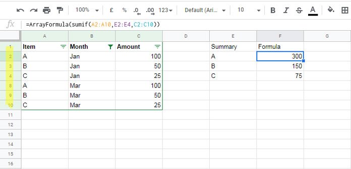
Screenshot of regular SUMIF with ArrayFormula in Google Sheets showing totals that include hidden rows in filtered data

You’ve now filtered out all rows for February. But if you check the previous SUMIF result, you’ll notice no change—it still sums values from all rows, including the hidden ones.

That’s because SUMIF doesn’t respect filtered views.

Why Not Use SUMIFS?

In the post SUMIF Excluding Hidden Rows in Google Sheets (linked earlier), we used a helper column and a SUMIFS formula to exclude hidden rows when working with a single criterion.

But here, we’re working with multiple items (A, B, C) and want the results in an expanding array using ArrayFormula. Unfortunately, SUMIFS doesn’t work with ArrayFormula like SUMIF does.

So what’s the solution?

Applying SUMIF with ArrayFormula to Filtered Rows

To make SUMIF respect filter views, we need to modify the formula so it only considers visible rows. Here’s how.

Final Formula

=ArrayFormula(SUMIF(
   A2:A10&"|"&MAP(C2:C10, LAMBDA(r, SUBTOTAL(103, r))), 
   E2:E4&"|"&1, 
   C2:C10
))

Animated GIF showing SUMIF with ArrayFormula using MAP and SUBTOTAL to return totals based only on visible (filtered) rows in Google Sheets

Only the visible months—Jan and Mar—are included in the totals. Rows for Feb are correctly ignored.

How the Formula Works

SUBTOTAL(103, r) returns 1 for visible rows and 0 for hidden ones.
MAP(..., LAMBDA(...)) applies this visibility check to each row in the sum range.
Each Item value is combined with its row visibility using "|", forming keys like "A|1" or "B|0".
The criteria range is similarly adjusted with "|1" to match only visible rows.
The sum range C2:C10 remains unchanged.
This ensures that only visible rows matching each item are summed—without needing helper columns.

Conclusion

While SUMIF doesn’t support filtered data by default, this workaround using ArrayFormula, MAP, and SUBTOTAL allows you to sum only visible rows without needing helper columns. It’s a practical way to use SUMIF with ArrayFormula for filtered data in Google Sheets, especially when you’re working with multiple criteria.

If you try to replicate this with SUMIFS, it becomes more complex—you’d need to use multiple LAMBDA functions: one to add the visibility flag and another to repeat SUMIFS for each criterion. That can make your formula resource-intensive, especially in large datasets.

This approach offers a cleaner, more efficient alternative when dealing with filtered data and multiple conditions.

Want more ways to work with filtered or visible rows in Google Sheets? Try these: