In a filtered table range, how do you determine the current or longest winning/losing/tie streaks in Google Sheets?

For example, you have three columns in your table for Player 1, Player 2, and Winners, respectively. You may need to find the winning and losing streaks between two players or the current streak of the winner/loser/tie.

Given the multitude of players, filter two players in both the Player 1 and Player 2 columns, and then compute the longest winning, losing, tie streaks, or the current streak.

We can achieve this in Google Sheets, and below are the formulas (for the first time, I believe). Before that, here are my tutorials that help you find streaks in unfiltered columns:

1. Longest Winning and Losing Streak Formulas in Google Sheets
2. Finding Current Win/Loss Streak in Google Sheets

Using FILTER: Sample Data and Application

We have the sample data in A1:C, where A1:C1 contains the field labels Player 1, Player 2, and Winner, respectively.

It contains four unique players: Adam, Bella, Charlie, and Dylan.

We will filter Adam and Bella in column A and then in column B. Subsequently, we will obtain the winners’ names in column C. If the game results in a tie, it will be represented by the letter T, instead of the winner’s name.

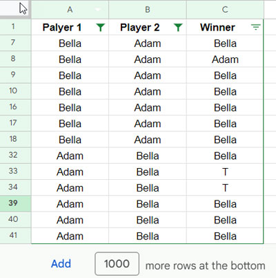
Once filtered, we will use column C to find the longest winning streak of Adam, the losing streak of Adam (which will be the longest winning streak of Bella), and the longest tie streak.

Additionally, we will find the current streak with the name.

You can likewise filter other names and observe the streaks without making any changes in the formulas, except for the players.

Since the sample data is spread across several rows (51 rows), I suggest you copy my sample sheet by clicking the button below.

Sample Sheet

Filtering Data:

If you are using your own data, filter it according to the following instructions; however, my sample data is already filtered.

Select columns A to C and click on Data > Create a filter.

Then click on the drop-down in cell A1, and click on “clear”. This will clear all the selected names. Then select the names Adam and Bella and click OK.

Click on the drop-down on cell B1 and select the said two names accordingly.

Now, let’s navigate to the formulas to identify the winning, losing, or tie streaks in the data from column C within the filtered table.

Longest Winning/Losing/Tie Streaks in a Filtered Data Range in Google Sheets

We will start with finding the longest winning streak of player Adam in our filtered table.

Formula:

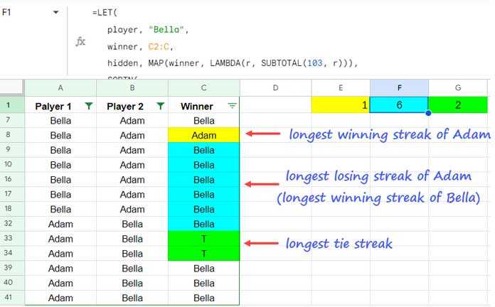
=LET(
   player, "Adam", 
   winner, C2:C, 
   hidden, MAP(winner, LAMBDA(r, SUBTOTAL(103, r))), 
   SORTN(
      FREQUENCY(
         IF((winner=player)*hidden, ROW(winner)), 
         IF((winner=player)+(hidden=0), ,ROW(winner))
      ), 1, 0, 1, 0
   )
)

To find the longest losing streak in the filtered data range, replace “Adam” with the other player name, which is “Bella”.

To find the longest tie streak in the filtered range, replace “Adam” with the text that you used to represent a draw in the winner column, which is “T” in my case.

When applying this formula to an alternative filtered data range in your sheet, aside from the player name, simply substitute C2:C with the appropriate winner column reference.

As per my sample data, the formula will return 1, 6, and 2 as the longest winning, losing, and tie streaks in the filtered data, respectively.

Formula Explanation

The formula is not overly complex. It’s a bit lengthy as I used the LET function to name value expressions, making it easier to avoid repetitive calculations and edit the formula.

As you can see, you only need to edit the player name and winner column reference in the formula in one place.

Syntax of the LET Function:

LET(name1, value_expression1, [name2, …], [value_expression2, …], formula_expression)

Names and Value Expressions in the Formula:

• player is the name “Adam”
• winner is the column reference C2:C
• hidden is MAP(winner, LAMBDA(r, SUBTOTAL(103, r))) which returns the count 1 in visible rows and 0 in hidden rows by evaluating the values in the rows in the winner column.

This MAP and SUBTOTAL combo helps us exclude filtered-out rows (including only visible rows) in the longest winning, losing, and tie streaks in the formula expression part. Please check my SUBTOTAL guide for more info.

Formula Expression:

SORTN(
      FREQUENCY(
         IF((winner=player)*hidden, ROW(winner)), 
         IF((winner=player)+(hidden=0), ,ROW(winner))
      ), 1, 0, 1, 0
   )

SORTN(…, 1, 0, 1, 0): The SORTN function is employed to get the max value in the FREQUENCY output.

Syntax: SORTN(range, [n], [display_ties_mode], [sort_column], [is_ascending], [sort_column2, …], [is_ascending2, …])

Where range is the FREQUENCY result, n (number of rows in the result after sorting) is 1, display_ties_mode is 0, sort_column is 1, is_ascending is 0 (descending order).

FREQUENCY( IF((winner=player)*hidden, ROW(winner)), IF((winner=player)+(hidden=0), ,ROW(winner)) ): It returns the frequency distribution.

Syntax: FREQUENCY(data, classes)

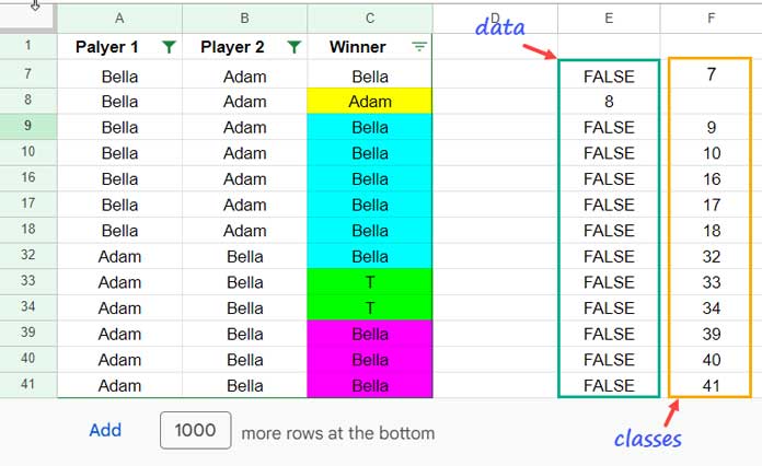
data: IF((winner=player)*hidden, ROW(winner)) – It returns the row number of player “Adam” in matching visible rows. winner=player returns either TRUE or FALSE. Multiplying that with 1 or 0 returns 1 in visible rows and 0 in hidden rows. The IF formula returns the row number wherever the logical expression returns 1; else, it returns FALSE.

Classes: IF((winner=player)+(hidden=0), ,ROW(winner)) – It returns blanks in rows wherever C2:C="Adam" or hidden is equal to 0, and row numbers in all other rows.

The longest winning, losing, and tie streaks in the filtered range are determined by the maximum value in the frequency distribution. This calculation relies on the specified player value.

Current Winning/Losing/Tie Streak in Filtered Data Range in Google Sheets

Understanding the current winning/losing/tie streak in the filtered data is relatively easy.

It represents the occurrence of the last value in the winner column (after filtering players in columns A and B) from bottom to top until there is a change in the value.

Formula:

=ArrayFormula(LET(
   winner, C2:C, 
   hidden,  MAP(winner, LAMBDA(r, SUBTOTAL(103, r))), 
   range, FILTER(winner, hidden=1), 
   val, CHOOSEROWS(range, -1), 
   test, range=val, 
   data, IF(test, SEQUENCE(ROWS(range))), 
   classes, IF(test, ,SEQUENCE(ROWS(range))), 
   current_streak, CHOOSEROWS(FREQUENCY(data, classes), -1), 
   HSTACK(val, current_streak)
))

Formula Breakdown:

Below are the names and value expressions used in the formula that returns the current winning/losing/tie streak in the filtered data range in Google Sheets.

C2:C: The assigned name is winner.

MAP(winner, LAMBDA(r, SUBTOTAL(103, r))) – returns 1 in visible rows and 0 in hidden rows. The assigned name is hidden.

FILTER(winner, hidden=1) – it filters C2:C, excluding hidden rows. The assigned name is range.

CHOOSEROWS(range, -1): it (CHOOSEROWS) returns the last value in the range. The assigned name is val. With the current filtering, the formula will yield the name “Bella.”

range=val: this logical expression matches val (“Bella”) in range and returns TRUE for matches and FALSE for mismatches. The assigned name is test.

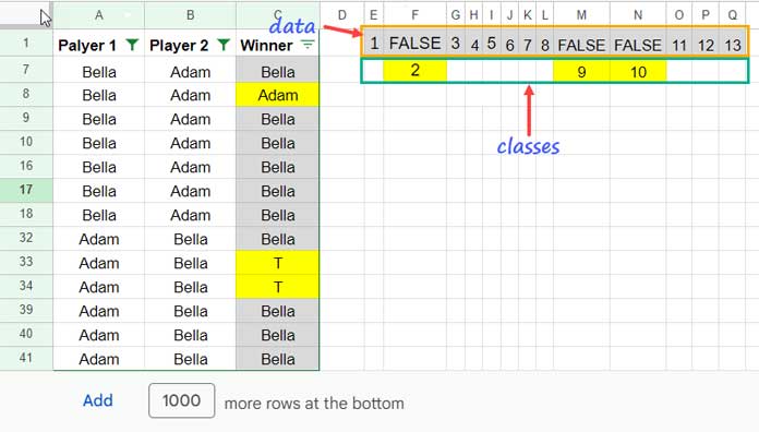
IF(test, SEQUENCE(ROWS(range))): logical test to return sequence numbers if the test evaluates to TRUE; otherwise, it returns FALSE. In other words, it generates sequence numbers against “Bella” in visible rows, and otherwise returns FALSE. The assigned name is data.

IF(test, ,SEQUENCE(ROWS(range))): it returns blank if the test evaluates to TRUE, else sequence numbers. The assigned name is classes.

The screenshot below illustrates the data and classes, presented horizontally for clarification:

CHOOSEROWS(FREQUENCY(data, classes), -1): returns the current streak, which is the last value in the FREQUENCY result. The assigned name is current_streak.

Here is the formula expression:

HSTACK(val, current_streak) – horizontally stacks the current streak value with the corresponding player name. It can be “Adam”, “Bella”, or “T” as per our sample data. With the current filtering, the formula will return {"Bella", 3}.

The formula requires two horizontal cells to return the result.

Conclusion

In conclusion, the methods outlined for calculating winning, losing, and tie streaks in a filtered range within Google Sheets provide a powerful and flexible approach.

Leveraging the combination of LET, MAP, SUBTOTAL, FREQUENCY, and various other functions enables precise tracking of streaks based on players’ filtering.

Whether determining the longest streaks or the current streak in a filtered dataset, these formulas offer a versatile solution for analyzing game outcomes in a dynamic and organized manner.

Moreover, the formulas will respond seamlessly when the filter is removed. They are designed to work equally well in both filtered and unfiltered datasets, ensuring consistent and reliable streak analysis.