Understanding the current winning or losing streak is important when managing sports or gaming data in Google Sheets. In a previous guide, we talked about finding the longest streaks.

In this tutorial, we’ll show you how to easily find and calculate your current winning and losing streaks using Google Sheets. We’ll mainly use the FREQUENCY function, along with other functions, to get the results you need.

The provided formula aims to give you a clear picture of performance trends, helping you make well-informed decisions based on your data.

For practice, we’ll work with data in column A, range A3:A, skipping any empty cells while looking at the current win/loss streak.

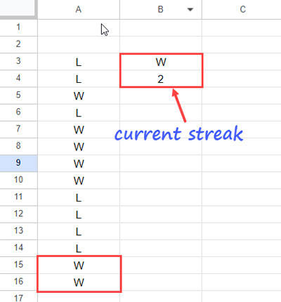
In our example, ‘W’ stands for ‘Win,’ and ‘L’ stands for ‘Loss.’ However, feel free to replace ‘W’ and ‘L’ with different values, like game or player names, to match your specific situation.

How to Find Current Win/Loss Streak in Google Sheets

For the sample data above, you can use the following formula to find the winning or losing streak:

=ArrayFormula(LET(
   winner, TOCOL(A3:A, 1), 
   val, CHOOSEROWS(winner, -1), 
   test, winner=val, 
   data, IF(test, SEQUENCE(ROWS(winner))), 
   classes, IF(test, ,SEQUENCE(ROWS(winner))), 
   current_streak, CHOOSEROWS(FREQUENCY(data, classes), -1), 
   VSTACK(val, current_streak)
))

First, a detailed explanation of this formula will be provided. Following that, you can learn how to modify this formula using the BYCOL lambda to return the current streaks of multiple columns of data.

Formula Explanation

The formula employs the LET function to assign name with the results of value_expression and returns the outcome of the formula_expression, representing the current win/loss streak.

Syntax:

LET(name1, value_expression1, [name2, …], [value_expression2, …], formula_expression)

Note: Assigning names can enhance the formula’s efficiency because the value_expressions are evaluated only once in the LET function.

Below are the names, value expressions, and their roles:

• TOCOL(A3:A, 1): TOCOL returns the range after removing blank cells. The assigned name is winner.
• CHOOSEROWS(winner, -1): CHOOSEROWS returns the last value in winner. The assigned name is val.
• winner=val: Matches val in winner and returns TRUE for matches and FALSE for mismatches. The assigned name is test.
• IF(test, SEQUENCE(ROWS(winner))): IF logical test to return sequence numbers if the test is TRUE; otherwise, it returns FALSE. The assigned name is data. Please refer to Column B in the image below.
• IF(test, ,SEQUENCE(ROWS(winner))): Returns blank if test = TRUE, else sequence numbers. The assigned name is classes. Please refer to Column C in the image below.
• CHOOSEROWS(FREQUENCY(data, classes), -1): The key part that returns the current winning or losing streak. The assigned name is current_streak.

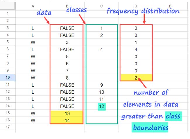
We use the FREQUENCY function in Google Sheets to return the frequency distribution of a one-dimensional array into specified classes. The array here is represented by data, and classes are represented by classes.

The output of FREQUENCY will be a range of size one greater than the number of elements in the classes (Please refer to Column D in the image above).

The final value is the number of elements in data greater than any of the class boundaries. That value will be the current streak value. We have employed CHOOSEROWS to extract the value.

• VSTACK(val, current_streak): The formula which appends val. It will be ‘W’ if the current streak is a winning streak, else “F.”

Finding Current Win/Loss Streaks Across Multiple Sets of Data

Sometimes, you may have multiple sets of data and want to find the current winning or losing streak for each of them separately.

Of course, you can copy-paste the formula and replace the ranges. However, you can use a single formula to return the current winning/losing streaks for multiple sets of data at once.

For example, if the data is in A3:C and we want the current winning/losing streaks of A3:A, B3:B, and C3:C separately, let’s use the BYCOL lambda for this.

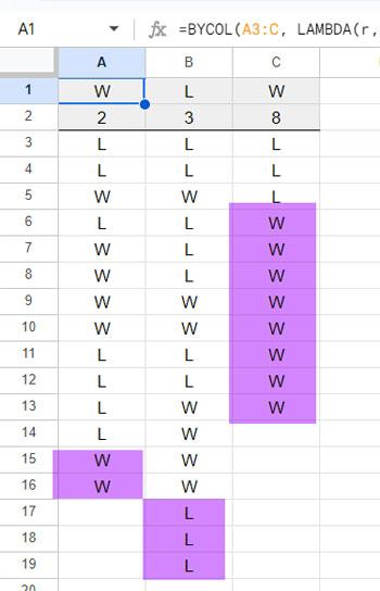
Generic Formula: BYCOL(A3:C, LAMBDA(r, current_streak_formula))

In the current_streak_formula, you need to replace A3:C (winner) with r.

Formula:

=BYCOL(A3:C, LAMBDA(r, 
   ArrayFormula(LET(
      winner, TOCOL(r, 1), 
      val, CHOOSEROWS(winner, -1), 
      test, winner=val, 
      data, IF(test, SEQUENCE(ROWS(winner))), 
      classes, IF(test, ,SEQUENCE(ROWS(winner))), 
      current_streak, CHOOSEROWS(FREQUENCY(data, classes), -1), 
      VSTACK(val, current_streak)
   )))
)

Resources

In conclusion, mastering the art of finding the current win/loss streak in Google Sheets opens up a wealth of analytical possibilities. For further exploration, here are a few more related resources.

1. Winning/Losing/Tie Streaks in a Filtered Range in Google Sheets
2. Highlight Data Spikes (Consecutive Increases) in Google Sheets
3. Highlight N Consecutive Decreases in Numeric Data in Google Sheets
4. Get the Count of Consecutive Occurrences of Values in Google Sheets
5. Consecutive Dates to Date Ranges in Google Sheets: The REDUCE Method
6. Get the Most Frequent Keywords from Titles in Google Sheets
7. How to Filter the Top 3 Most Frequent Strings in Google Sheets