This post outlines the steps for highlighting N consecutive decreases in a numeric data column or row within Google Sheets.
Navigating through this somewhat complex challenge, we will tackle it by employing an array formula in a designated helper column or row.
This array formula will serve as the basis for highlighting the corresponding data column or row. The highlighting process will be executed using an XLOOKUP-based formula rule.
Recognizing the importance of such conditional formatting is pivotal in data analysis with Google Sheets.
Effectively identifying and highlighting instances of N consecutive decreases in numeric data provides valuable insights into trends and patterns.
We will begin by highlighting three consecutive decreases and later switch to N.
How to Highlight Three Consecutive Decreases in a Column in Google Sheets
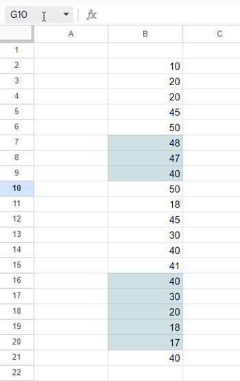
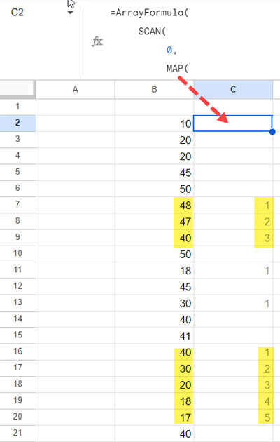
For example purposes, we will use the range B2:B, which contains numeric data. In cell C2, enter the following formula:
=ArrayFormula(
     SCAN(
          0,
          MAP(
               INDIRECT("B2:B"&XMATCH("?*", B:B&"", 2, -1)),
               LAMBDA(r, IF(r-OFFSET(r, -1, 0)>=0, ,1))
          ),
          LAMBDA(a, v, IF(v=0, , a+v))
     )
)
I’ll explain the formula later on.
Note: When you use this formula, replace B2:B with the column range that contains the numbers to highlight, and replace B:B with the column reference. For example, if you want to highlight A10:A, replace B2:B with A10:A and B:B with A:A. No other changes are required.
Now, let’s apply the highlighting rule to B2:B to highlight three consecutive decreases in this numeric data range.
- Click on Format > Conditional formatting.
- In the “Apply to range,” enter B2:B.
- Select “Custom formula” under “Format rules” and enter the following highlight rule:
=XLOOKUP(3, C2:C4, C2:C4, , 1, -1) - Choose your preferred formatting style and click “Done.”
This will highlight all three consecutive decreases in column B (cell range B2:B) in Google Sheets.
Note: If your range to highlight is A10:A and the helper column range is B10:B, replace C2:C4 (both occurrences) in the XLOOKUP with B10:B12. No other changes are required.
How to Convert Three Consecutive Decreases to N?
You just need to modify the highlighting rule; there’s no need to adjust the formula in the helper column.
The XLOOKUP formula above is crafted to identify three consecutive decreases using the values in the helper column.
Syntax:
XLOOKUP(search_key, lookup_range, result_range, [missing_value], [match_mode], [search_mode])Where in the formula:
search_key= 3lookup_range= C2:C4result_range= C2:C4missing_value= nullmatch_mode= 1search_mode= -1
To highlight three consecutive decreases, I’ve applied the formula to the first three values in C2:C, specifically the cell range C2:C4.
The formula searches for the value 3 in the range from the last value to the first value and returns the value that is 3 or greater than 3. To understand it, enter the XLOOKUP in cell D2 and copy-paste it down.
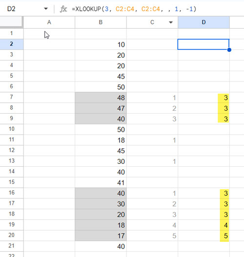
Within conditional formatting, the formula automatically expands down in the applied range and highlights wherever it evaluates a value.
To highlight four consecutive decreases, utilize the range C2:C5 as the lookup and result range with the lookup value set to 4.
For instance, to highlight five consecutive decreases in sequence, use the following XLOOKUP formula in Conditional formatting:
=XLOOKUP(5, C2:C6, C2:C6, , 1, -1)Anatomy of the Helper Formula
a. Dynamic Range Part:
We implemented a dynamic range instead of B2:B in the formula, structured as follows:
INDIRECT("B2:B"&XMATCH("?*", B:B&"", 2, -1))When used with ARRAYFORMULA, it adapts to the range B2:B21, as illustrated in my example. The range automatically expands when a value is entered below B21. XMATCH identifies the last non-blank cell in column B.
In this context, B2:B represents the range to highlight N consecutive decreasing values, while B:B refers to the entire column.
b. MAP and OFFSET Part:
The MAP function processes the dynamic range, iterating over each value in the array. We use ‘r’ to define each value within the lambda function.
The lambda function, specifically IF(r-OFFSET(r, -1, 0)>=0, ,1), subtracts the value in the current row from the value in the previous row. If the difference is >=0, the formula returns null; otherwise, it returns 1.
This results in a column with 1s and blanks, where a cell containing 1 indicates a decrease in value.
c. SCAN Part:
The SCAN function requires an initial value and an array. The initial value is 0, and the array is the result of the MAP and OFFSET operations. ‘a’ is used to define the accumulator value, and ‘v’ defines each value in the array.
The lambda function within SCAN, IF(v=0, , a+v), essentially returns a running sum, visible in the helper column.
We use this output to highlight N consecutive decreases in a column in Google Sheets.
How to Highlight Three Consecutive Decreases in a Row in Google Sheets
If the data is arranged in a row, you may need to adjust both the highlight rule and the helper column formulas. There are minor changes in both formulas.
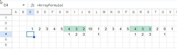
Assuming you want to highlight three consecutive decreases in the row range C3:3, here are the required changes in the formulas:
Helper Formula in cell C4 (for Highlighting N Consecutive Decreasing Values in a Row):
=ArrayFormula(
     SCAN(
          0,
          MAP(
               INDIRECT("C3:"&ADDRESS(3, XMATCH("?*", 3:3&"", 2, -1))),
               LAMBDA(r, IF(r-OFFSET(r, 0, -1)>=0, ,1))
          ),
          LAMBDA(a, v, IF(v=0, , a+v))
     )
)
Highlight Rule (for Highlighting 3 Consecutive Decreasing Values in a Row):
=XLOOKUP(3, C4:E4, C4:E4, , 1, -1)You can apply this rule to the “Apply to range” C3:3.
To highlight N consecutive decreasing values, you can follow the earlier approaches. For example, the following formula will highlight 5 consecutive decreasing values in the range C3:3:
=XLOOKUP(5, C4:G4, C4:G4, , 1, -1)Changes in the Formulas
The major change is in the array used within the MAP, which is now represented as INDIRECT("C3:"&ADDRESS(3, XMATCH("?*", 3:3&"", 2, -1))).
In this case, C3 is the starting cell to highlight, and 3:3 represents the row to highlight.
Unlike the formula used for columns, here we utilize the ADDRESS function because we need to find the cell address of the last column with a value in row #3. In the previous example, finding the row number was sufficient.
Another modification is in the OFFSET part of MAP. Previously, we used the function to offset by one row; here, we need to offset by 1 column.
Regarding the highlight rule, which is XLOOKUP, there are no changes. You need to perform the lookup in the row instead of a column.
Conclusion
This tutorial covers highlighting N consecutive decreases in Google Sheets, from identifying the pattern to applying the conditional formatting.
Want to dive deeper? Explore more conditional formatting techniques in the Ultimate Guide to Conditional Formatting in Google Sheets.


