Before highlighting the smallest N values in a row—or in each row—you should decide how to handle duplicates and ties at the Nth position. The table below outlines the options:
| Value | Strictly Lowest N | Lowest N + Ties of Nth | Distinct Lowest N |
| 1 | ✅ | ✅ | ✅ |
| 1 | ✅ | ✅ | |
| 2 | ✅ | ✅ | ✅ |
| 2 | ✅ | ||
| 3 | ✅ |
Here are the custom formula rules to highlight the smallest N values in a row or each row in Google Sheets.
Rule 1: Strictly Lowest N in a Row or Each Row
=AND(LEN(B2), XMATCH(CELL("address", B2), SORTN(TOCOL(ADDRESS(ROW($B2:$J2), COLUMN($B2:$J2))), 3, 0, TOCOL($B2:$J2), TRUE)))This formula highlights the smallest N values in each row, excluding ties at the Nth position.
Replace $B2:$J2 with your desired row range, B2 with the first cell in the range, and 3 with your preferred N value.
You can apply this to a single row (e.g., $B2:$J2) or multiple rows (e.g., $B2:$J8) without modifying the formula. Just update the “Apply to range” field accordingly in the Conditional Formatting Rules panel.
Example:
- Select the range
B2:J8 - Go to Format > Conditional formatting
- Under Format rules, select Custom formula is, and paste the formula
- Choose a formatting style and click Done
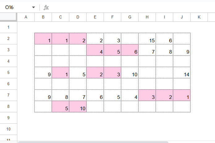
How it works:
TOCOL(ADDRESS(ROW($B2:$J2), COLUMN($B2:$J2)))returns the cell addresses of each value in the row.SORTN(..., 3, 0, TOCOL($B2:$J2), TRUE)gives the addresses of the lowest 3 values.XMATCHchecks if the current cell’s address is among them.ANDensures the cell isn’t blank and that it’s one of the lowest 3.
This works row-by-row because the formula uses absolute column references and relative row references.
Rule 2: Lowest N + Ties of Nth in a Row or Each Row
=RANK(B2, $B2:$J2, TRUE)<=3Use this to highlight the lowest 3 values plus any values tied at the 3rd lowest spot.
Update $B2:$J2 with the first row of your data and B2 with the first cell in that row.
Follow the same steps as in Rule 1 to apply this rule.
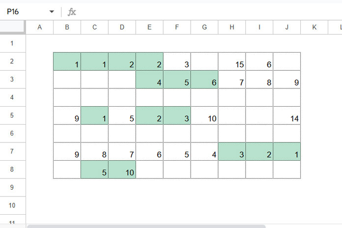
How it works:
- The
RANKfunction assigns the smallest value a rank of 1, the next smallest 2, and so on. - Tied values share the same rank, and subsequent ranks skip accordingly.
- All cells with rank ≤3 get highlighted.
Rule 3: Distinct Lowest N in a Row or Each Row
=AND(XMATCH(B2, SORTN(TOCOL($B2:$J2), 3, 2, 1, TRUE)), COUNTIF($B2:B2, B2)=1)Use this to highlight the smallest 3 distinct values in each row—ignoring duplicates.
Replace $B2:$J2 with the first row in your data, B2 with the first cell, and $B2:B2 with a corresponding range.
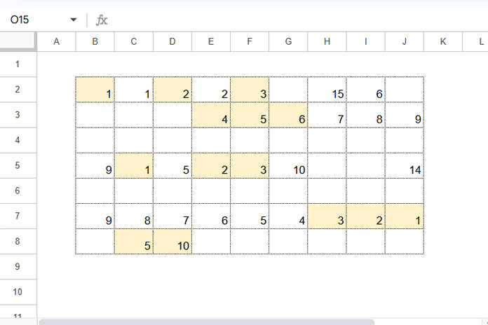
How it works:
SORTN(TOCOL($B2:$J2), 3, 2, 1, TRUE)returns the smallest 3 unique values.XMATCH(B2, ...)checks if the current cell is among them.COUNTIF($B2:B2, B2)=1ensures only the first occurrence of each value is considered.ANDreturns TRUE only if both conditions are met.
Conclusion
This tutorial showed multiple ways to highlight the smallest N values in each row in Google Sheets. Depending on your requirement—strictly N values, including ties, or distinct values—you can choose the formula that best fits your dataset.
For more advanced conditional formatting techniques, explore The Ultimate Guide to Conditional Formatting in Google Sheets, which includes 80+ tutorials covering a wide range of real-world use cases.


