Without relying on a helper column, we can calculate the longest winning, losing, and tie streaks in Google Sheets. To achieve this, we will utilize a combination of ROW, LEN, IF, FREQUENCY, and SORTN functions.

Before diving into the main example, let’s first explore a simpler example using the helper column approach. This approach is particularly helpful for users who are new to Google Sheets.

Let’s consider a scenario where two players participated in a Chess championship and played ten games consecutively.

Player 1’s results are outlined below, where 0 represents a loss, 0.5 indicates a tie/draw, and 1 signifies a win (please refer to cells B2:B11 in image#1 below).

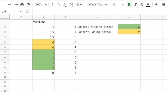
To determine the longest winning streak, utilize the IF logical test below in cell C2 and copy-paste it into cells C3:C11.

=IF(B2=1, 1+C1, 0)

Then, employ the MAX function in any blank cell:

=MAX(C2:C11)

For the longest losing streak, replace the logical test in cell C2 with the following one and copy-paste it into cells C3:C11:

=IF(B2=0, 1+C1, 0)

No changes are needed in the MAX function. What about tie/draw?

Use =IF(B2=0.5, 1+C1, 0) in C2 to create the helper column. Ensure to drag this formula down to cell C11.

All the formulas above require an empty cell C1.

That’s all about the non-array helper column approach. Now, let’s move on to the array formulas part.

Longest Win, Draw, or Loss Streak: Array Formulas in Google Sheets

I am in favor of using array formulas for the said calculation to avoid occupying additional cells (helper columns).

Please disregard the formulas in column C. Instead, input the following array formula into cell E2.

Winning Streak Array Formula (E2):

=SORTN(
   FREQUENCY(
      IF((B2:B=1)*LEN(B2:B), ROW(B2:B)), 
      IF((B2:B=1)*LEN(B2:B), , ROW(B2:B))
   ), 1, 0, 1, 0
)

The above formula calculates the values in the range B2:B and displays the longest winning streak in cell E2 in Google Sheets.

To determine the longest losing streak, you only need to make two changes. Replace (B2:B=1) with (B2:B=0) (appearing twice in the formula).

Losing Streak Array Formula (E3):

=SORTN(
   FREQUENCY(
      IF((B2:B=0)*LEN(B2:B), ROW(B2:B)), 
      IF((B2:B=0)*LEN(B2:B), , ROW(B2:B))
   ), 1, 0, 1, 0
)

To determine the longest draw/tie streak, representing the longest consecutive series of draws or ties, use (B2:B=0.5) instead.

Draw/Tie Array Formula (E4):

=SORTN(
   FREQUENCY(
      IF((B2:B=0.5)*LEN(B2:B), ROW(B2:B)), 
      IF((B2:B=0.5)*LEN(B2:B), , ROW(B2:B))
   ), 1, 0, 1, 0
)

Yes! The B2:B=1 in the win formula changes to B2:B=0 in the loss formula, and B2:B=0.5 in the draw formula.

Formula Explanation

Let’s begin with the generic formula for E2/E3/E4, which is as follows:

Generic Formula:

=SORTN(
   FREQUENCY(
      data, 
      classes
   )
)

We have employed two logical tests to retrieve the data and classes, which we will delve into in detail later in this tutorial.

As mentioned, all the array formulas for win/draw/loss streaks above are identical. They are composed of a combination of the functions ROW, LEN, IF, FREQUENCY, and SORTN.

SORTN Part:

=SORTN(
   FREQUENCY(
      data, 
      classes
   )
)

The purpose of the SORTN function here is to virtually sort the output of the FREQUENCY function in descending order and return the topmost row value. In simpler terms, it extracts the maximum value.

The crucial element of the longest win/loss/tie streak formula in Google Sheets is the FREQUENCY function.

FREQUENCY Part: The Key Formula in Longest Win/Draw/Loss Streak Calculation

=SORTN(
   FREQUENCY(
      data, 
      classes
   )
)

A basic understanding of the FREQUENCY function is essential for learning the longest winning streak in Google Sheets.

For instance, we’ve applied the following SEQUENCE formula in cell G1 to generate numbers 1 to 10 in G1:G10:

=SEQUENCE(10)

Then, using =FREQUENCY(G1:G10, {3, 8}) in H1, we obtain 3, 5, and 2 in H1, H2, and H3, respectively.

• data – G1:G10
• classes – {3, 8}

This implies that the count of inputs in G1:G10 less than or equal to 3 is 3, between 4 and 8 (both inclusive) is 5, and above 8 is 2.

Now, let’s return to our Chess championship example in Google Sheets.

In our longest winning streak formula in cell E2, the data and classes in the FREQUENCY function are as follows (highlighted):

• data – =ArrayFormula(IF((B2:B=1)*LEN(B2:B), ROW(B2:B)))
• classes – =ArrayFormula(IF((B2:B=1)*LEN(B2:B),,ROW(B2:B)))

Note: The ArrayFormula function is not required in the master formula as SORTN can replace it.

I’ve entered them in cells D2 and E2 for explanation purposes, as shown in the screenshot.

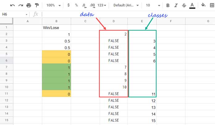
If we use the FREQUENCY formula, i.e., =FREQUENCY(D2:D11, E2:E11), it will return {1, 0, 0, 0, 4, 0}.

This means:

• The count of elements in the data range D2:D11 less than or equal to 3 is 1 (in Google Sheets, the FREQUENCY function excludes FALSE values when counting the occurrences of values within a range).
• >3 and <=4 is 0.
• >4 and <=5 is 0.
• >5 and <=6 is 0.
• >6 and <=11 is 4.
• Above 11 is 0.

The maximum value is 4, which represents the winning streak. We can use SORTN to retrieve that, and that’s what I have implemented in our E2, E3, and E4 master formulas.

For the longest losing streak and tie streak formulas, the data and classes are slightly different. I’ll address that in the logical part below.

Logical Part (IF, ROW, and LEN):

=SORTN(
   FREQUENCY(
      data, 
      classes
   )
)

The IF logical component determines the data and classes for the FREQUENCY, playing a pivotal role in calculating the longest win/loss/tie streak in Google Sheets.

LEN is employed to skip blank cells in rows.

In the longest winning streak formula:

• For data, the logical test returns the row numbers of the rows containing 1 (refer to image#2 D2:D11).
• Regarding classes, the logical test returns the row numbers of the rows not containing 1 (refer to image#2 E2:E11).

For the longest losing streak formula:

• data = row numbers of cells containing 0.
• classes = row numbers of cells not containing 0.

For Tie Streak:

• data = row numbers of cells containing 0.5.
• classes = row numbers of cells not containing 0.5.

Resources

In addition to finding the longest win, loss, and tie streaks, you may also be interested in determining the current win or loss streak. The formula varies slightly compared to the ones mentioned above, although it still utilizes the FREQUENCY function. You can explore that tutorial and other related resources below.

• Finding Current Win/Loss Streak in Google Sheets
• Winning/Losing/Tie Streaks in a Filtered Range in Google Sheets
• Highlight Data Spikes (Consecutive Increases) in Google Sheets
• Highlight N Consecutive Decreases in Numeric Data in Google Sheets
• Get the Count of Consecutive Occurrences of Values in Google Sheets
• How to Filter the Top 3 Most Frequent Strings in Google Sheets