Calculating the weighted average of filtered or visible data in Google Sheets requires a workaround. Why is that?

The SUMPRODUCT and AVERAGE.WEIGHTED functions, though popular for weighted average calculations, do not natively exclude hidden rows.

To overcome this, we can identify visible rows using a combination of the SUBTOTAL and MAP functions in an array formula, creating a virtual helper column within the existing formulas.

Regular Weighted Average Calculation

Before filtering or hiding rows, let’s revisit the standard weighted average formula:

Weighted Average = Sum(Data_Point_Value × Weight) ÷ Sum(Weight)

For example, assume we procure different quantities of a product at different unit prices.

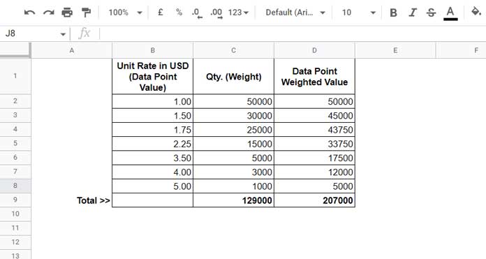
Example Calculation:

Weighted Average = Sum(Data_Point_Value × Weight) ÷ Sum(Weight)

=207,000 ÷ 129,000 = 1.60 USD

In Google Sheets, the following formulas can be used for this calculation:

Formula #1: Using AVERAGE.WEIGHTED

Syntax: AVERAGE.WEIGHTED(values, weights)

=AVERAGE.WEIGHTED(B2:B8, C2:C8) 

Formula #2: Using SUMPRODUCT

Syntax: SUMPRODUCT(values, weights) / SUM(weights)

=SUMPRODUCT(B2:B8, C2:C8) / SUM(C2:C8) 

Calculating the Weighted Average of Filtered Data

Now, let’s exclude specific rows (e.g., rows 6, 7, and 8) from the calculation without deleting them. Instead, we’ll hide these rows using filtering, grouping, manual hiding, or slicers.

The issue is that the above formulas will still include hidden rows because they cannot distinguish between visible and hidden rows.

To resolve this, the first step is to identify visible rows using the SUBTOTAL and MAP functions.

Identifying Visible Rows:

The following formula will return 1 for visible rows and 0 for hidden rows:

=MAP(C2:C8, LAMBDA(r, SUBTOTAL(103, r)))

Adjusting Formulas to Exclude Hidden Rows in Weighted Average Calculations

Here’s how to modify the formula to exclude hidden rows:

Using AVERAGE.WEIGHTED

Generic Formula:

INDEX(AVERAGE.WEIGHTED(values, weights * visible_rows_identifier))

Example Formula:

=INDEX(AVERAGE.WEIGHTED(B2:B8, C2:C8 * MAP(C2:C8, LAMBDA(r, SUBTOTAL(103, r)))))

This modification multiplies the weights by the MAP and SUBTOTAL combo, setting weights of hidden rows to 0.

Using SUMPRODUCT

Similarly, you can modify the SUMPRODUCT formula as follows:

Generic Formula:

SUMPRODUCT(values, weights, visible_rows_identifier) / SUMPRODUCT(weights * visible_rows_identifier)

Example Formula:

=SUMPRODUCT(B2:B8, C2:C8, MAP(C2:C8, LAMBDA(r, SUBTOTAL(103, r)))) / SUMPRODUCT(C2:C8 * MAP(C2:C8, LAMBDA(r, SUBTOTAL(103, r))))

This workaround effectively excludes hidden rows from the calculation of a weighted average in Google Sheets.

Thanks for reading! Enjoy!

Resources

• Calculate the Average of Visible Rows in Google Sheets
• Weighted Moving Average in Google Sheets (Formula Options)
• AVERAGE Function: Advanced Tips and Tricks in Google Sheets
• How to Use the TRIMMEAN Function in Google Sheets
• How to Use the HARMEAN Function in Google Sheets
• GEOMEAN for Geometric Mean Calculation in Google Sheets
• DAVERAGE Function in Google Sheets: Formula Examples