The HARMEAN function in Google Sheets, categorized under statistical functions, returns the harmonic mean of a dataset. This type of mean is especially useful for calculating the average of rates, such as speed or ratios.
What Is the Harmonic Mean?
To understand the HARMEAN function, you first need to understand the concept of reciprocals. This is because the harmonic mean is calculated as the reciprocal of the arithmetic mean of the reciprocals of the dataset.
Here’s the general formula:
Harmonic Mean = n / (1/x₁ + 1/x₂ + 1/x₃ + ... + 1/xₙ)
Where:
- n is the number of data points
- x₁, x₂, …, xₙ are the data values
This makes the harmonic mean especially useful when the values are rates or ratios (e.g., speeds, prices per unit, etc.).
Example Calculation
Let’s take three values: 1, 3, and 5.
Using the formula manually:
=3 / (1/1 + 1/3 + 1/5)
=3 / (1 + 0.3333 + 0.2)
=3 / 1.5333 ≈ 1.957
Instead of calculating this manually, you can use the built-in HARMEAN function in Google Sheets.
HARMEAN Function Syntax
HARMEAN(value1, [value2, ...])Arguments:
value1: (Required) The first value or range to include in the dataset.value2: (Optional) Additional individual values or ranges to include.
Examples
Example 1: Single Range
To calculate the harmonic mean of values in B2:B4 (which contain 1, 3, and 5):
=HARMEAN(B2:B4)This returns approximately 1.957.
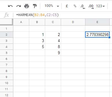
Example 2: Multiple Ranges
Assume:
B2:B4contains: 1, 3, 5C2:C5contains: 2, 4, 8, 9
You can combine both ranges in a single formula:
=HARMEAN(B2:C5)This computes the harmonic mean across all the values in the two-column range.
Handling Errors
Common Error: #NUM!
The HARMEAN function in Google Sheets will return an error error if:
- Any numeric value in the range is less than or equal to zero – harmonic mean is undefined for zero or negative values.
- All values in the range are non-numeric, leaving no valid numbers to calculate the mean.
- The range contains error values (like
#DIV/0!,#VALUE!, etc.) from other formulas.
Important:
The function ignores text and blank cells automatically. These do not cause errors and are simply excluded from the calculation.
To safely handle error values in your data, you can wrap the input range with IFERROR:
=HARMEAN(IFERROR(C2:C5))When to Use the HARMEAN Function in Google Sheets
Use the HARMEAN function when you need a more accurate average of rates or ratios. For example:
- Average speed over different segments of a journey
- Average price per unit when quantity varies
- Financial metrics like P/E ratios
It’s especially effective when extremely high or low values would otherwise distort a standard arithmetic average.
Related Articles
- How to Use the TRIMMEAN Function in Google Sheets
- GEOMEAN for Geometric Mean Calculation in Google Sheets
- AVERAGE Function: Advanced Tips and Tricks in Google Sheets
- AVERAGEIF Function for Conditional Averages in Google Sheets
- AVERAGEIFS Multiple Criteria Function in Google Sheets
- How to Calculate a Weighted Average in Google Sheets
- DAVERAGE Function in Google Sheets: Formula Examples


