In this tutorial, I’ll walk you through how to use the OR logic in multiple columns in COUNTIFS in Google Sheets.
For conditional counting, it’s easy to use multiple OR conditions (this or that) in one column. For example, we want to count column D if the text in that column is “painting” or “driving.”
In that case, we can use the below ARRAYFORMULA, SUM, and COUNTIFS combination.
Formula # 1 – Correct ✔
=ARRAYFORMULA(SUM(
   COUNTIFS(
      D:D, {"Driving", "Painting"}
   )
))
However, the same trick may not work in multiple columns. I understand you need an explanation for this. Here you go!
Assume you want to extend the above formula to one more column. That is, count column E for favorite authors “Leo Tolstoy” and “Jane Austen” from among a bunch of authors.
The following formula is not going to work!
Formula # 2 – Incorrect ✖
=ARRAYFORMULA(SUM(
   COUNTIFS(
      D:D, {"Driving", "Painting"},
      E:E, {"Leo Tolstoy", "Jane Austen"}
   )
))
Using OR in multiple columns in COUNTIFS is quite tricky in Google Sheets. We have seen a workaround solution already: COUNTIFS with Multiple Criteria in the Same Range in Google Sheets.
However, the limitation is that it is not flexible enough to use a criteria range. That approach is best for hardcoding the criteria within the formula.
Here, we will use REGEXREPLACE for applying OR logic in multiple columns in the COUNTIFS function.
Using REGEXREPLACE for OR Logic in Multiple Columns with COUNTIFS
We have seen two COUNTIFS formulas above – one working and another non-working. Here is the sample data used in those formulas in the range B1:E.
| Name | Gender | Hobby | Favorite Author |
| Amy | F | Painting | Leo Tolstoy |
| Pamela | F | Driving | Agatha Christie |
| Misty | F | Driving | Leo Tolstoy |
| Jessica | F | Driving | Agatha Christie |
| Kevin | M | Painting | Jane Austen |
| Martin | M | Painting | Agatha Christie |
| Tim | M | Fishing | Jane Austen |
| Albert | M | Fishing | Agatha Christie |
First of all, we will rewrite formula #1, which is already returning the correct result, using our new method.
That will help us rewrite the non-working formula #2 easily. Before that, let’s understand the logic quickly.
REGEXREPLACE in COUNTIFS (Logic)
The first formula counts the text criteria “Driving” and “Painting” in column D.
Here we will substitute both criteria with a unique string, symbol, or character using REGEXREPLACE.
It’s up to you to choose the replacement text/character/symbol. In my example, I am going to use the character “A.”
Then, using COUNTIFS, we will count the criterion “A” instead of the multiple OR criteria, i.e., “Driving” and “Painting.”
Syntax:
COUNTIFS(criteria_range1, criterion1, [criteria_range2, …], [criterion2, …])Note: The arguments within the square brackets are optional, and we don’t need them in our formula #1.
Generic Formula # 1:
ARRAYFORMULA(
   COUNTIFS(
      regexreplace_formula_1, "A"
   )
)criteria_range1–regexreplace_formula_1criterion1–"A"
If there is one more column, we will do the substitution in that column also. But, the criteria will be substituted with another value, for example, “B.”
Generic Formula # 2:
ARRAYFORMULA(
   COUNTIFS(
      regexreplace_formula_1, "A",
      regexreplace_formula_2, "B"
   )
)
Let’s apply OR in multiple columns in COUNTIFS.
Formula Examples
Here is the replacement of Formula #1 as per Generic Formula #1.
One Column:
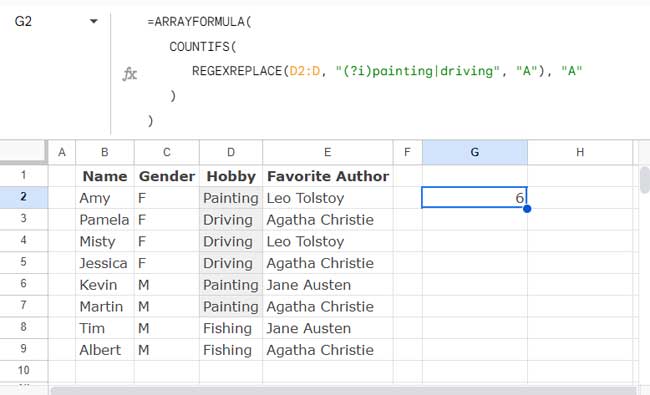
=ARRAYFORMULA(
   COUNTIFS(
      REGEXREPLACE(D2:D, "(?i)painting|driving", "A"), "A"
   )
)
If you want to add more conditions, separate each one with a pipe. For example, to include “Fishing,” replace (?i)painting|driving with (?i)painting|driving|fishing.
Formula #2 as per Generic Formula #2 (it’s the replacement of our non-working formula given at the top of this tutorial).
Two Columns:
ARRAYFORMULA(
   COUNTIFS(
      REGEXREPLACE(D2:D, "(?i)painting|driving", "A"), "A",
      REGEXREPLACE(E2:E, "(?i)Leo Tolstoy|Jane Austen", "B") , "B"
   )
)
What about OR logic in a third column in COUNTIFS?
I know, now you can do that yourself. I am leaving the generic formula for you to make it easier.
Three Columns:
ARRAYFORMULA(
   COUNTIFS(
      regexreplace_formula_1, "A",
      regexreplace_formula_2, "B",
      regexreplace_formula_3, "C"
   )
)
COUNTIFS OR Logic in Multiple Columns and Criteria Range Usage
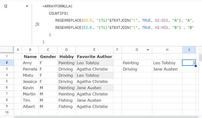
This time we have the criteria, i.e., the hobbies “painting” and “driving” in G2:G3, and the favorite authors, i.e., “Leo Tolstoy” and “Jane Austen” in H2:H3.
In that case, what you need to do is to combine them and separate with a pipe delimiter using the TEXTJOIN function as follows:
=ARRAYFORMULA(
   COUNTIFS(
      REGEXREPLACE(D2:D, "(?i)"&TEXTJOIN("|", TRUE, G2:G3), "A"), "A",
      REGEXREPLACE(E2:E, "(?i)"&TEXTJOIN("|", TRUE, H2:H3), "B") , "B"
   )
)
This approach will help you include several criteria when applying OR logic in the COUNTIFS function in Google Sheets.
Resources
- Google Sheets: COUNTIFS with Not Equal to in Infinite Ranges
- COUNTIFS in a Time Range in Google Sheets [Date and Time Column]
- Not Blank as a Condition in COUNTIFS in Google Sheets
- COUNTIF | COUNTIFS Excluding Hidden Rows in Google Sheets
- How To Use COUNTIF or COUNTIFS In Merged Cells In Google Sheets
- Varying Array Sizes in COUNTIFS in Google Sheets
- OR in COUNTIFS in Either of the Columns in Google Sheets
- COUNTIFS with ISBETWEEN in Google Sheets
- Counting XLOOKUP Results with COUNTIFS in Excel and Google Sheets


Great! I found this very useful. Thank you for such an elaborate post.