RANK.AVG is a statistical function. One hurdle in ranking is the repeated numbers. The RANK.AVG function in Google Sheets is useful in such situations.
Similar to the RANK function, the RANK.AVG can also return the rank of a specified value or values in a range. But there is one difference. The RANK function returns the same rank for repeated numbers but the RANK.AVG finds the average of the repeated ranks and returns it.
There is no function in Google Sheets that you can use as a tiebreaker in Ranking. If you want continues ranks for repeated numbers, I have a custom formula.
Similar: Ranking without duplicates in Google Sheets.
Now let me explain to you how to use the RANK.AVG function in Google Sheets.
Syntax and Examples to the Use of the RANK.AVG Function in Google Sheets
Syntax:
RANK.AVG(value, data, [is_ascending])
Here value is the value whose rank that you want to find in a set of data.
Don’t forget to specify, by using TRUE or FALSE, whether you want to rank the value in ascending order or descending order.
If you skip, the RANK.AVG formula in Google Sheets would return the rank in descending order as it’s the default setting. I will detail this in the examples below.
You should note one more thing. The value can also be an array. You can use the function ArrayFormula with RANK.AVG for this.
Examples to the Use of RANK.AVG Function in Google Sheets
In the below two examples, I have used the RANK formula. Not the RANK.AVG formula. This’s because there is no duplicate value in Column A.
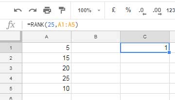
Example 1: Basic Formula.

Here you can use the RANK.AVG formula too and that also would return the same result.
=RANK.AVG(25,A1:A5)
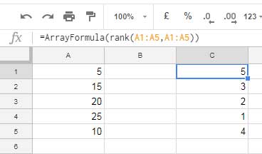
Example 2: Array Formula.

Here again the RANK.AVG formula can return the same result.
=ArrayFormula(RANK.AVG(A1:A5,A1:A5))
When you go through the ranks, you can see that the max value in Column A, which is 25, got the 1st rank.
You can reverse that by specifying TRUE at the end of the formula as below.
=ArrayFormula(RANK.AVG(A1:A5,A1:A5,TRUE))
There are 5 numbers in column A. This time the rank of the value 25 would be 5th.
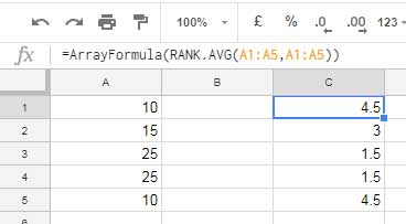
Now let me show you one example with duplicate numbers in Column A. So that you can understand the real use of the RANK.AVG Function in Google Sheets.

In the above example, the number 10 and 25 repeats twice. See their ranks. If you want, you can get the rank of the value 25 using the non-array formula as below.
=RANK.AVG(25,A1:A5)
The normal RANK formula would return the rank 1 for both the values in cell A3 and A4. The RANK.AVG formula returns 1.5 for both.
Prepare a sample sheet as above and repeat a number more than 2 times in Column A. Then you can understand the pattern of the Rank average.
If the highest number repeats twice, there is an addition of 0.5 with the actual rank. If it’s thrice, the addition with the original rank would be 1. This pattern continues.
If the lowest number repeats there is a subtraction of 0.5 for each repetition as above. That’s all about the RANK.AVG function in Google Sheets. Enjoy!


