The RANK.EQ function in Google Sheets returns the rank of a number within a given dataset. It’s a statistical function that works the same as the older RANK function.
Is there any difference between the two functions?
No — they produce the same results. You can use either one, but I recommend using RANK.EQ instead of RANK, as the latter exists mainly for backward compatibility.
The “EQ” in RANK.EQ stands for Equal. This means that if two or more numbers in the dataset are the same, they will receive the same (equal) rank, and a gap will appear in the ranking sequence where the tie occurs.
If you want to return the average rank instead of assigning the same rank to duplicates, use RANK.AVG. However, there’s no built-in way to break ties without writing a custom formula — I’ve covered that in my tutorial How to Rank Without Ties in Google Sheets.
The easiest way to understand how RANK.EQ works is to use it on a sorted list of numbers. By doing so, you can clearly see:
- The rank of a number corresponds to its position in the dataset.
- You can rank either from largest to smallest or from smallest to largest.
Sorting the dataset isn’t required — RANK.EQ works regardless of order — but sorting can make the results easier to interpret. You’ll see this in the examples below.
RANK.EQ Function Syntax in Google Sheets
This function is straightforward to learn and has only three arguments (the third is optional).
Syntax:
RANK.EQ(value, data, [is_ascending])- value – The number whose rank you want to determine (e.g., the value in cell A1 when ranking A1:A10).
- data – The list of numbers in an array or range (e.g., A1:A10). Non-numeric values are ignored.
- is_ascending – (Optional) Determines ranking order:
FALSE(default): Ranks in descending order, so the largest value gets rank 1.TRUE: Ranks in ascending order, so the smallest value gets rank 1.
RANK.EQ Function Example in Google Sheets
Suppose A2:A3 contains:
25
50
40
- In descending order (
FALSE): ranks are 3, 1, and 2. - In ascending order (
TRUE): ranks are 1, 3, and 2.
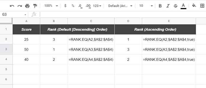
By default (in B2:B4), the preferred method is descending order so that the top value gets rank 1. Ascending order (in D2:D4) reverses this.
Tip: When copying the formula down a column:
- Use an absolute reference (e.g.,
$A$2:$A$11) for thedatarange. - Use a relative reference (e.g.,
A2) for thevaluecell.
This prevents errors when dragging the formula.
Example formula:
=RANK.EQ(A2, $A$2:$A$11, TRUE)In this example, TRUE means the smallest value gets rank 1. Duplicate scores (e.g., A3:A4) will share the same rank.
If you use FALSE instead:
=RANK.EQ(A2, $A$2:$A$11, FALSE)…the largest value will get rank 1, and duplicates will still share ranks.
Using RANK.EQ with ArrayFormula in Google Sheets
RANK.EQ works with ArrayFormula, letting you return ranks for an entire column in one go.
Following the earlier example, enter this in B2:
=ARRAYFORMULA(IFNA(RANK.EQ(A2:A, A2:A, TRUE)))Important:
- Clear column B first to avoid
#REF!errors. - This formula uses an open range (A2:A), so it will return
#N/Afor blank rows. The IFNA function replaces those errors with blanks.
That’s all about how to use the RANK.EQ function in Google Sheets. Thanks for reading — enjoy!
Resources
- Rank Without Duplicates in Google Sheets
- How to Rank Group Wise in Google Sheets in Sorted or Unsorted Group
- Compare and Highlight Up and Down in Ranking in Google Sheets
- Highlight Top 10 Ranks in Single or Each Column in Google Sheets
- How to Rank Data by Alphabetical Order in Google Sheets
- How to Rank Text Uniquely in Google Sheets
- How to Use RANK IF in Google Sheets (Conditional Ranking)
- Rank per Group in Excel
- How to Break RANK Ties Alphabetically in Google Sheets


