Want to assign unique ranks even when values are tied? You can do that in Google Sheets by combining the RANK.EQ function with COUNTIF or COUNTIFS.

In this tutorial, I’ll show you how to rank without ties in Google Sheets, both with regular formulas and with an array formula.

Google Sheets provides two ranking functions:

• RANK.EQ
• RANK.AVG

However, neither of these functions can break ties on their own.

So when two or more values are the same, both functions return duplicate ranks:

• RANK.EQ assigns the same rank to tied values.
• RANK.AVG assigns the average of the tied ranks.

That doesn’t mean ranking without ties in Google Sheets is impossible.

We can easily create a rank without duplicates by combining RANK.EQ with COUNTIF.

This method also works as an array formula, allowing the results to spill automatically.

To make the logic easier to understand, I’ll start with the non-array (drag-down) version.

Rank Without Ties in Google Sheets (Non-Array Formula)

We can assign ranks in two ways:

1. Top to Bottom (Descending Order)

In descending order, the highest value in the dataset gets rank 1.

For example:

• Score 100 → Rank 1
• Score 99 → Rank 2

This is the most commonly used ranking method, such as ranking students based on marks or players based on scores.

2. Bottom to Top (Ascending Order)

In ascending order, the lowest value in the dataset gets rank 1.

For example:

• Time 99 seconds → Rank 1
• Time 100 seconds → Rank 2

This method is commonly used in competitions such as races, where the participant with the shortest time ranks first.

We usually follow the top to bottom (descending) approach.

So let’s start with that.

Top to Bottom Ranking (Descending Order)

In the example above, players Karen and Kristi both scored 5.

Using the regular ranking formula in cell D2:

=RANK.EQ(C2,$C$2:$C$9,0)

Then copy it down.

Formula Syntax:

RANK.EQ(value, data, [is_ascending])

Where:

• C2 → the value to rank (relative reference)
• $C$2:$C$9 → the dataset (absolute reference)
• 0 → descending order

The value reference should remain relative so it changes as you drag down, while the data range should remain fixed.

Break Ties and Assign Unique Ranks

To rank without ties, use this formula in E2 and copy it down:

=RANK.EQ(C2,$C$2:$C$9,0)+COUNTIF($C$2:C2,C2)-1

Please scroll up and refer to Image 1.

How COUNTIF Works Here

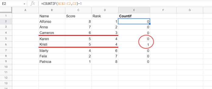
The COUNTIF part returns:

• 1 for the first occurrence
• 2 for the second occurrence
• 3 for the third occurrence

Since we subtract 1, it effectively adds:

• 0 to the first occurrence
• 1 to the second occurrence
• 2 to the third occurrence

This breaks the ties and gives each row a unique rank.

Bottom to Top Ranking (Ascending Order)

In some scenarios—such as races, lap timings, or speed competitions—the lowest value should rank first.

For example:

• Time 9.8 sec → Rank 1
• Time 10.1 sec → Rank 2

If tied values occur, use the following formulas.

In D2:

=RANK.EQ(C2,$C$2:$C$9,1)

In E2:

=RANK.EQ(C2,$C$2:$C$9,1)+COUNTIF($C$2:C2,C2)-1

Then copy both formulas down.

The only difference from the earlier formula is:

• 1 instead of 0

This tells Google Sheets to rank in ascending order.

Array Formula to Rank Without Ties in Google Sheets

If you don’t want to drag formulas down manually, use this array formula instead.

Unlike the non-array version, here we use COUNTIFS instead of COUNTIF.

Enter this formula in E2:

=ARRAYFORMULA(
   IFNA(
      RANK.EQ(C2:C9,C2:C9,0)+
      COUNTIFS(C2:C9,C2:C9,ROW(C2:C9),"<="&ROW(C2:C9))
      -1
   )
)

Refer to Image 1 above.

This formula automatically spills the results down.

Important:
If cells below contain existing values, Google Sheets will return a #REF! error.

This version ranks in descending order (highest value gets rank 1).

Array Formula for Ascending Ranking

If you want the lowest value to get rank 1, use:

=ARRAYFORMULA(
   IFNA(
      RANK.EQ(C2:C9,C2:C9,1)+
      COUNTIFS(C2:C9,C2:C9,ROW(C2:C9),"<="&ROW(C2:C9))
      -1
   )
)

Formula Explanation

This formula has two parts.

Part 1: Generate Base Rankings

RANK.EQ(C2:C9,C2:C9,0)

or

RANK.EQ(C2:C9,C2:C9,1)

This returns the rank of each value.

Part 2: Count Occurrences

COUNTIFS(C2:C9,C2:C9,ROW(C2:C9),"<="&ROW(C2:C9))-1

This returns:

• 0 for the first occurrence
• 1 for the second occurrence
• 2 for the third occurrence

Adding this to the rank values removes duplicates in ranking.

If the COUNTIFS part looks new to you, I’ve explained it in detail in my Running Count in Google Sheets tutorial.

Alternative Method

As a side note, I also have another array-based approach for ranking without duplicate ranks.

While RANK.EQ + COUNTIFS is the simplest method, you may also want to check:

Rank Without Duplicates in Google Sheets

That’s all about how to rank without ties in Google Sheets.

Thanks for staying with me. Enjoy!

Resources

• How to Break RANK Ties Alphabetically in Google Sheets
• How to Use RANK IF in Google Sheets (Conditional Ranking)
• How to Rank Group Wise in Google Sheets in Sorted or Unsorted Group