Unlike Excel, you can use the RANK function together with the FILTER function to rank group wise in Google Sheets.

In group wise ranking, there should be two columns – one column contains the group names and the second column contains the numbers to rank.

Also, it’s not necessary that the group of data is sorted in any order. Let’s see how to rank group wise in Google Sheets.

Rank Group Wise in Google Sheets (Rank Within Group)

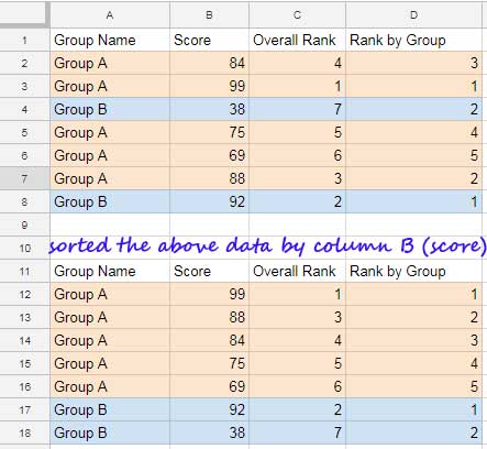
Here is my sample data in the range A1: D8. In this, the first column contains the group and the second column the numbers to rank.

There are two groups in the column A. They are “Group A”, and “Group B”. You can include as many groups as you want.

I have my below formula to Rank by Group in cell D2 which is then copied to the range D3: D8.

The Formula to Rank Group Wise in Google Sheets: 

=Rank(B2,Filter(B$2:$B$8,A$2:$A$8=A2),0)

To make you understand the difference between overall ranking and group-wise ranking, below the original data, you can see the sorted data included in the range A11: D18.

In that the sorting is based on the score, that is column B. Take a look at the results in column D in this sorted range.

Additional Notes:

The greatest value in each group will have the rank 1. If you want the lowest value having the rank 1, change the last parameter in the formula from 0 to 1. See that formula below.

=Rank(B2,Filter(B$2:$B$8,A$2:$A$8=A2),1)

Hope you could understand now how to rank group wise in Google Sheets.

RANK + Filter Combo Formula Explanation

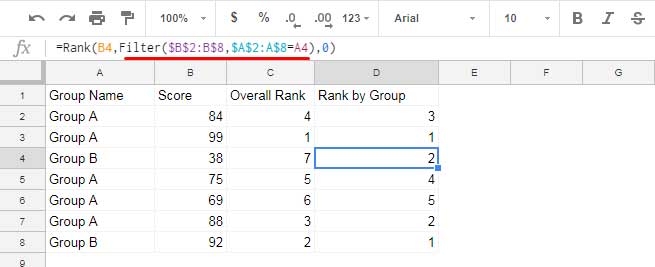
When you copy or drag the formula in cell D2 down, the formula changes as below. For example, here is the formula in cell D4.

The formula filters column B if the values in column A is “Group B”. For this row, the filter output will be the numbers 38 and 92.

That means, for this row # 4, you can read the Rank formula as below which returns the rank 2.

=rank(38,{38;92},0)

Conclusion

The RANK + FILTER combination has an advantage over the conventional SUMPRODUCT based formula which is popular among Excel users.

You can easily change the ranking order by changing the last parameter in the formula from 0 to 1 or 1 to 0.

Finally, you can use the same above formula even if your category in column A is not sorted.