Find the Rank of an Item in Each Column in Google Sheets

How to find the rank of an item based on its position in each column in Google Sheets?

I hope the topic above will be interesting for many of you! Let me give you a basic idea of the topic prior to further proceeding.

For example, I have given a list containing the name of four food items to three users/customers and requested them to rank those food items.

Later, I have prepared a table in Google Sheets, as per their feedback/ranking, as below.

Rank	Tom	Clara	Michael
1	Maryland crabcakes	Sourdough bread	Cornbread
2	Sourdough bread	Tater Tot	Sourdough bread
3	Cornbread	Cornbread	Tater Tot
4	Tater Tot	Maryland crabcakes	Maryland crabcakes

Now I want to check the rank of an item, for example, “Maryland crabcakes”, in each column in this table in Google Sheets.

Since the number of items is only 4 and the users are limited to 3, we can easily find the ranks manually. It would be as follows.

1] Tom

4] Clara

4] Michael

We can automate the same with a formula in Google Sheets. So that we can find the rank of several items based on their position in each column in Google Sheets.

See what I am talking about. As per my example, the food items are in F2:F5 and their ranks are in the next 3 columns.

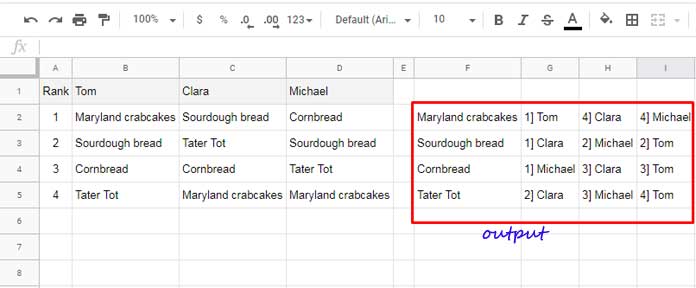
Finding the Rank of an Item in Each Column in Google Sheets

Are you interested in this? Then follow the steps below.

Steps to Find the Rank of an Item in Each Column in Google Sheets

There are four (main) steps involved in finding the rank of items in each column in Google Sheets. You can find them under different subtitles below.

I will start writing the formula in cell G2 the result of which will expand to adjoining columns and rows. In each step, I’ll modify this formula to reach the final formula.

1. Match an Item in Multiple Columns in Google Sheets

We can use the REGEXMATCH function to match an item in multiple columns in Google Sheets.

For example, If we use the following REGEXMATCH formula in the above list, the result would be a table with TRUE | FALSE values.

=ArrayFormula(regexmatch($B$2:$D$5,F2))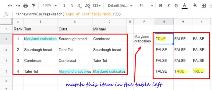

Match an Item in Multiple Columns - Regex over Match

The REGEXMATCH regular expression formula returns TRUE, wherever the item “Maryland crabcakes” matches in the table left.

2. Find the Position of an Item in Each Column in Google Sheets

To find the rank of the above item in each column first we must get the position of it in each column. For that, we can use a combination formula. Of course, the above REGEXMATCH will be a part of it.

Some of you may ask, why I am not using the MATCH function to find the position. The answer is MATCH is for a single column or row.

If we use MATCH, for three users, we must use three MATCH formulas combined as below in a single cell or individually in three different cells. Here is the combined one for your reference.

={match($F$2,B2:B5,0),match($F$2,C2:C5,0),match($F$2,D2:D5,0)}

We can’t easily modify this formula or not practical to use if there are more users/columns. So I am using a different approach.

I am just going to convert the TRUE values to the corresponding relative position. For that, I am making use of the ADDRESS function as below in Google Sheets.

=ArrayFormula(if(regexmatch($B$2:$D$5,F2)=true,regexextract(address(row($A$2:$A$5)-1,column($B$2:$D$2)),"[0-9]+"),))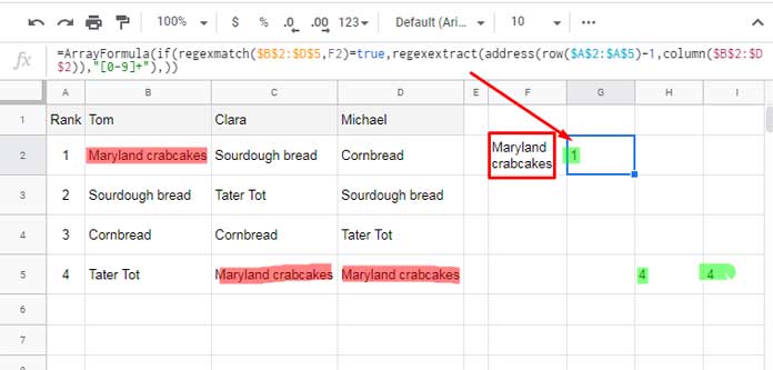

Sheets Formula to Find the Position of an Item in Each Column

Formula Explanation

You can see the value -1 used in the formula. It’s because of the range starts from the second row. If the range is B3:D6 instead of B2:D5, then change -1 to -2.

The ADDRESS formula address(row($A$2:$A$5)-1,column($B$2:$D$2)) within the above actually returns the cell addresses of the corresponding TRUE values in the range.

The REGEXEXTRACT wrapping it removes the unwanted strings and returns only the relative positions in multiple columns. You can refer to the screenshot above.

Join Scattered Cell Values and Split it to Single Row

The above rank of the item “Maryland crabcakes” in each column is scattered, right?

We just need to combine them and split to make it in a single row. Before that TRANSPOSE (change the data orientation) the above formula output. I’ll later tell you why this step is necessary.

=ArrayFormula(transpose(if(regexmatch($B$2:$D$5,F2)=true,regexextract(address(row($A$2:$A$5)-1,column($B$2:$D$2)),"[0-9]+"),)))

After this step, using TEXTJOIN, join the numbers and use the pipe as the separator.

=ArrayFormula(textjoin("|",true,(transpose(if(regexmatch($B$2:$D$5,F2)=true,regexextract(address(row($A$2:$A$5)-1,column($B$2:$D$2)),"[0-9]+"),)))))

Result in Cell G2: 1|4|4

Then SPLIT it to columns and done!

=ArrayFormula(split(textjoin("|",true,(transpose(if(regexmatch($B$2:$D$5,F2)=true,regexextract(address(row($A$2:$A$5)-1,column($B$2:$D$2)),"[0-9]+"),)))),"|"))

The Reson for Using TRANSPOSE before TEXTJOIN

You may now want to know why I have transposed the positions of the item before TEXTJOIN. Here is my answer!

In the next step, I’ll combine the user names with the above formula output. It (the user names) won’t match the ranking columns (SPLIT output) without transpose. Still having doubt, right?

See the below ‘new’ example to know how TEXTJOIN treats values (D1 and D2 outputs).

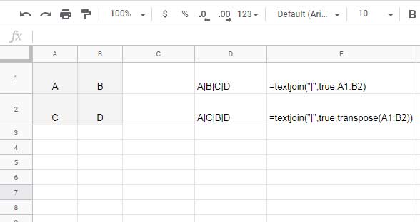
Reason for Using Transpose with Textjoin in Sheets

It first combines the values in the first row (A1:B1) and then the second row (A2:B2). You can see the same in cell D1.

But what we want is to combine values in the first column (A1:A2) and then the second column (B1:B2) as per the result in cell D2. Because we want to assign column header (user names) to ranks in corresponding columns.

The above ‘new’ example is just to make you understand the TEXTJOIN. So please ignore it hereafter in this tutorial.

3. Combine Column Header with Rank of an Item in Each Column

Just combine the name of the users (column header) with the above (cell G2 formula) using the CURLY BRACES which uses to form virtual arrays in Google Sheets. For that modify the G2 formula as below.

=ArrayFormula({split(textjoin("|",true,(transpose(if(regexmatch($B$2:$D$5,F2)=true,regexextract(address(row($A$2:$A$5)-1,column($B$2:$D$2)),"[0-9]+"),)))),"|");B1:D1})

The output will be what you are looking for.

1	4	4
Tom	Clara	Michael

We have now found the rank of the item “Maryland crabcakes” in each column in Google Sheets. But it has two issues. What are they?

We have not sorted the rank, though it’s not necessary for this item as it’s already in ascending order.
The output occupies two rows and three columns. We want this in one row only so that we can drag the formula down to find the rank of multiple items in each column in Google Sheets.

4. Sort the Rank of the Item in Ascending Order

We want to sort the rank, which is in the first row of the result. The SORT function in Google Sheets for sorting the columns, not rows. So first transpose the above output and then sort.

The Formula in Cell G2:

=sort(transpose({split(textjoin("|",true,(transpose(if(regexmatch($B$2:$D$5,F2)=true,regexextract(address(row($A$2:$A$5)-1,column($B$2:$D$2)),"[0-9]+"),)))),"|");B1:D1}))

Note: Removed the ARRAYFORMULA function as it’s not required with SORT.

Result:

1	Tom
4	Clara
4	Michael

Here are the final steps to find the rank of an item in each column in Google Sheets.

Using two INDEX formulas we can split the above columns into two – one with rank and the other with the names.

Rank:

=index(sort(transpose({split(textjoin("|",true,(transpose(if(regexmatch($B$2:$D$5,F2)=true,regexextract(address(row($A$2:$A$5)-1,column($B$2:$D$2)),"[0-9]+"),)))),"|");$B$1:$D$1})),0,1)

Names:

=index(sort(transpose({split(textjoin("|",true,(transpose(if(regexmatch($B$2:$D$5,F2)=true,regexextract(address(row($A$2:$A$5)-1,column($B$2:$D$2)),"[0-9]+"),)))),"|");$B$1:$D$1})),0,2)

Combine both these formulas placing &"] "& in between in cell G2.

=ArrayFormula(index(sort(transpose({split(textjoin("|",true,(transpose(if(regexmatch($B$2:$D$5,F2)=true,regexextract(address(row($A$2:$A$5)-1,column($B$2:$D$2)),"[0-9]+"),)))),"|");$B$1:$D$1})),0,1)&"] "&index(sort(transpose({split(textjoin("|",true,(transpose(if(regexmatch($B$2:$D$5,F2)=true,regexextract(address(row($A$2:$A$5)-1,column($B$2:$D$2)),"[0-9]+"),)))),"|");$B$1:$D$1})),0,2))

Then again TRANSPOSE.

=transpose(ArrayFormula(index(sort(transpose({split(textjoin("|",true,(transpose(if(regexmatch($B$2:$D$5,F2)=true,regexextract(address(row($A$2:$A$5)-1,column($B$2:$D$2)),"[0-9]+"),)))),"|");$B$1:$D$1})),0,1)&"] "&index(sort(transpose({split(textjoin("|",true,(transpose(if(regexmatch($B$2:$D$5,F2)=true,regexextract(address(row($A$2:$A$5)-1,column($B$2:$D$2)),"[0-9]+"),)))),"|");$B$1:$D$1})),0,2)))

You can refer to the image below for the output (G2:I2).

How to Find the Rank of Multiple Items Based on Position in Each Column in Google Sheets

Formula to Find the Rank of Multiple Items Based on Position in Each Column in Google Sheets

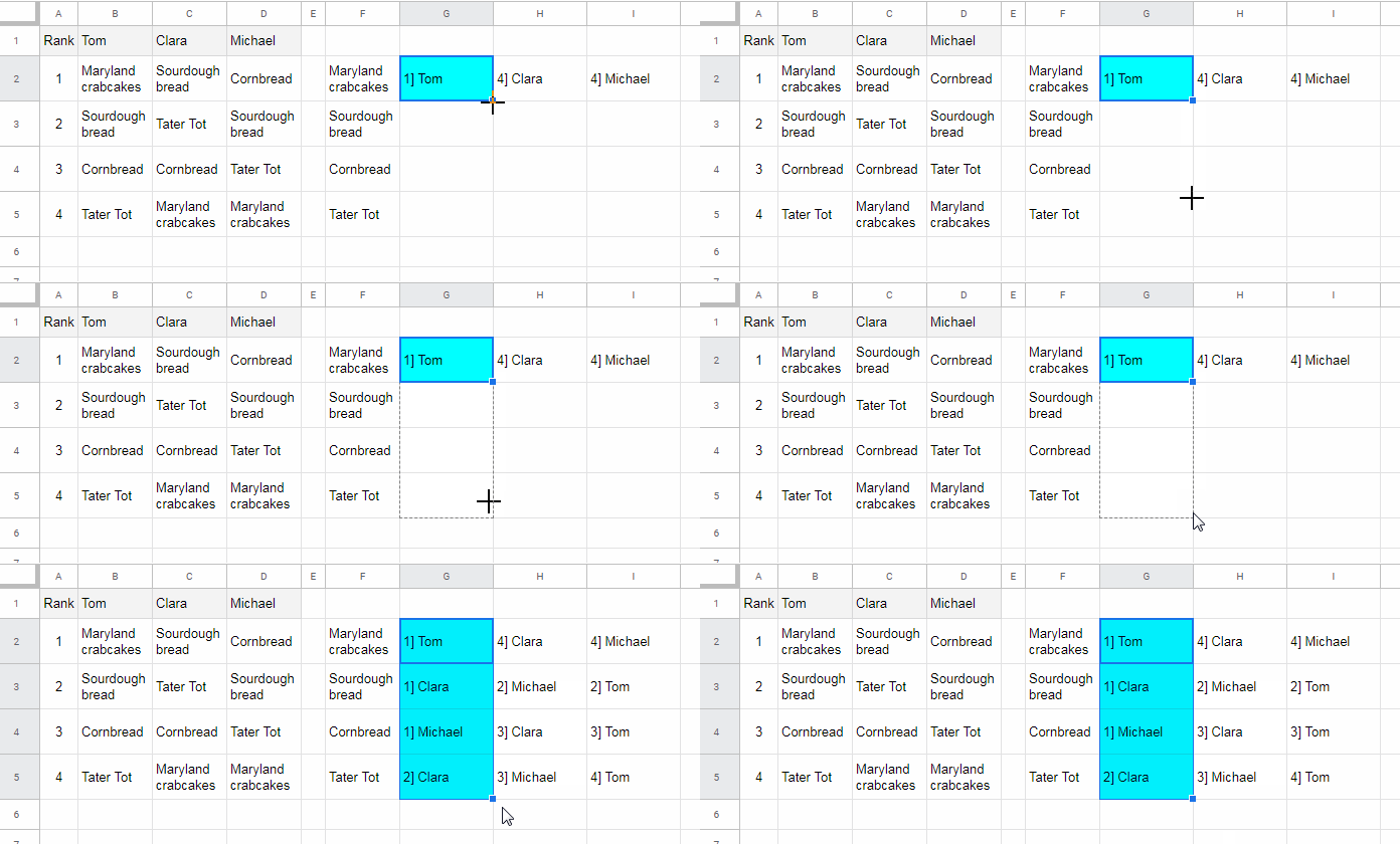
Steps:

Enter the item names in F2:F.
Drag the G2 formula down.

Usage Notes

The above formula is for the range B2:D5. To extend the number of rows (number of items), replace all the occurrence of $B$2:$D$5 in the formula with $B$2:$D and $A$2:$A$5 with $A$2:$A. Also, please do remove unused rows (blank rows) from the sheet.

If there are more users, for example, for 4 users, replace all the occurrence of $B$2:$D$2 in the formula with $B$2:$E$2.

The item must be unique in each column and must appear in each column. For example, if we want to find the rank of the item “Maryland crabcakes” in each column, for example, B to D, it must present in each column and must not repeat.