When your data spans more than one year and you want a summary month-wise, you will find the following step-by-step instructions useful.

In this tutorial, we will see how to write the best formula using SUMIF to sum by month and year in Google Sheets. You can even sort the summary in descending or ascending order based on the month and year column or the amount column.

The sample data is in two columns: B2:B and C2:C. The dates are in B2:B and the amounts to sum are in C2:C.

Before beginning, if your data is imported or entered by an inexperienced user, it’s better to test the correctness of the data. You can use functions like ISDATE to test if the date entry is valid and ISNUMBER to test if the entries in the amount column are valid.

That being said, let’s proceed to the step-by-step instructions for using SUMIF to sum data by month and year in Google Sheets.

Step 1: Getting Unique Beginning-of-Month Dates

Enter the following formula in cell E2 to return the unique beginning-of-the-month dates from the date range in B2:B:

=SORT(UNIQUE(EOMONTH(TOCOL(B2:B, 1), -1)+1), 1, TRUE)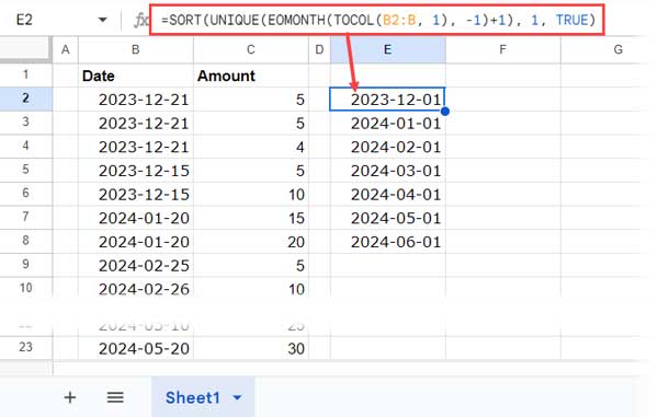

Before moving to the next step, let’s understand what each component in the formula does:

• TOCOL(B2:B, 1) – The TOCOL function removes blank cells in the range B2:B, returning only dates.
• EOMONTH(…, -1)+1 – This part of the formula converts the dates in column B to the end of the previous month, then adds 1 to shift them to the beginning of the current month.
• UNIQUE(…) – The UNIQUE function returns the unique beginning-of-the-month dates.
• SORT(..., 1, TRUE) – The SORT function sorts the unique beginning-of-the-month dates in ascending order.

The above formula returns the criteria for summing by month in chronological order. If you want the month and year to appear in descending order, replace TRUE in the last part of the formula with FALSE.

In the next step, we will format it to month and year.

Step 2: Formatting Beginning-of-Month Dates to Month and Year

Select the result in E2:E and, within the Format menu, click Number > Custom number format.

Enter “MMM-YY” for the month and year format, then click Apply.

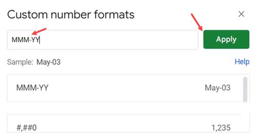
This formatting will change only the appearance; the underlying values in E2:E will still be the beginning-of-the-month dates.

With steps 1 and 2, we have completed the criteria needed to use a SUMIF function to return the sum of column C by month and year based on the date range in column B.

Step 3: Applying the SUMIF Formula to Sum by Month and Year

Enter the following SUMIF formula in cell F2 to sum by month and year:

=ArrayFormula(SUMIF(EOMONTH(B2:B, -1)+1, TOCOL(E2:E, 1), C2:C))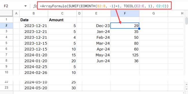

Formula Breakdown:

It follows the syntax SUMIF(range, criterion, [sum_range]).

• range: EOMONTH(B2:B, -1)+1 – This converts the dates in B2:B to the beginning of the month dates. This step is necessary because the criteria (from step 1) to test in this range are the beginning-of-the-month dates.
• criterion: TOCOL(E2:E, 1) – The TOCOL function removes blank cells in the criteria range E2:E.
• sum_range: C2:C – The range containing the values to sum.

With this formula, you can sum the values in column C by month and year based on the date range in column B.

Single Formula to Sum by Month and Year in Google Sheets

Above, we have two formulas: one in cell E2, which returns the criteria, and another in cell F2, which returns the sum by month and year.

We can combine them into a single formula as below:

=ArrayFormula(LET(
   criteria, UNIQUE(EOMONTH(TOCOL(B2:B, 1), -1)+1), 
   MonthlySum, SUMIF(EOMONTH(B2:B, -1)+1, TOCOL(criteria, 1), C2:C), 
   SORT(HSTACK(criteria, MonthlySum), 1, TRUE)
))

When you use this formula, replace B2:B with the date range and C2:C with the amount column range.

It will return a two-column output, and you should apply Format > Number > Custom number format > mmm-yy to the first column.

Formula Breakdown:

We have used the LET function to assign the name ‘criteria’ to the criteria formula and ‘MonthlySum’ to the sum by month and year formula. In the formula expression part of LET, we have used HSTACK to combine them.

Syntax of the LET Function:

LET(name1, value_expression1, [name2, …], [value_expression2, …], formula_expression)

Where:

• name1: criteria
• value_expression1: UNIQUE(EOMONTH(TOCOL(B2:B, 1), -1)+1)
• name2: MonthlySum
• value_expression2: SUMIF(EOMONTH(B2:B, -1)+1, TOCOL(criteria, 1), C2:C)
• formula_expression: SORT(HSTACK(criteria, MonthlySum), 1, TRUE)

Sorting the SUMIF Results by Month and Year or Amount

The formula currently sorts the first column (month and year) in ascending order. If you want to sort in descending order, replace TRUE in the formula expression part with FALSE.

If you want to sort the second column (amount) in descending order, replace 1 with 2 and TRUE with FALSE in the formula expression.

Here is the updated formula for sorting by month and year in descending order:

=ArrayFormula(LET(
   criteria, UNIQUE(EOMONTH(TOCOL(B2:B, 1), -1)+1), 
   MonthlySum, SUMIF(EOMONTH(B2:B, -1)+1, TOCOL(criteria, 1), C2:C), 
   SORT(HSTACK(criteria, MonthlySum), 1, FALSE)
))

And here is the updated formula for sorting the amount column in descending order:

=ArrayFormula(LET(
   criteria, UNIQUE(EOMONTH(TOCOL(B2:B, 1), -1)+1), 
   MonthlySum, SUMIF(EOMONTH(B2:B, -1)+1, TOCOL(criteria, 1), C2:C), 
   SORT(HSTACK(criteria, MonthlySum), 2, FALSE)
))

Resources

• Sum Data by Month (Not Year) in Google Sheets with SUMIF
• Creating Month Wise Summary in Google Sheets (Query Formula)
• Filter by Month and Year in Query in Google Sheets
• Create Daily, Weekly, Monthly, Quarterly, and Yearly Summaries in Google Sheets
• Sum Current Month Data Using Query Function in Google Sheets
• Rolling Months Backward Summary in Google Sheets