Knowing how to sum by quarter is crucial in Excel because quarterly reporting has become a standard practice in many industries.
For sum by quarter, we can leverage a regular SUMIFS formula, a dynamic array formula, or a custom function in Excel.
The basic SUMIFS formula requires users to input individual formulas for each quarter, making it easy to learn and use.
A dynamic array formula simplifies the process by allowing users to specify the year for which they want to generate quarterly reports, along with the date and amount ranges in the table. The formula returns the output in one step, making it more user-friendly.
The custom function, derived from the dynamic array formula, uses the same parameters but offers the advantage of being used just like a regular function. This function can be utilized across the entire workbook, enhancing efficiency and convenience.
Sample Data and Basic Formula
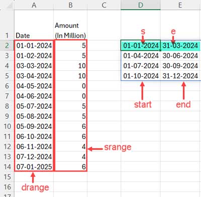
The table below, spanning cells A1:B14, presents projected cash flow dates in column A and amounts (in millions) in column B.
| Date | Amount (In Million) |
| 01-01-2024 | 5 |
| 01-02-2024 | 5 |
| 03-03-2024 | 10 |
| 03-04-2024 | 10 |
| 04-05-2024 | 0 |
| 04-06-2024 | 0 |
| 05-07-2024 | 5 |
| 05-08-2024 | 5 |
| 05-09-2024 | 6 |
| 06-10-2024 | 6 |
| 06-11-2024 | 4 |
| 07-12-2024 | 4 |
| 07-01-2025 | 6 |
As observed, the data spans two years, and our objective is to sum the cash flow amounts for each quarter within a specified year in Excel.
Therefore, we recommend using quarter start and end dates (e.g., 01/01/2024 to 31/03/2024) instead of specifying quarter numbers.
Step 1: Generating the Starting and Ending Dates for Each Quarter
In cell range D2:D5, enter the starting dates of each quarter.
In cell E2, enter the following formula to get the end date of the first quarter:
=EDATE(D2, 3)-1Navigate to cell E2, click, and drag the bottom-right fill handle down until cell E5.
Step 2: Applying the SUMIFS Formula for Quarterly Sums
Enter the following SUMIFS formula in cell F2 to return the sum of cash flow amounts in the first quarter:
=SUMIFS(
   $B$2:$B$14,
   $A$2:$A$14, ">="&D2,
   $A$2:$A$14, "<="&E2
)
This follows the syntax:
=SUMIFS(sum_range, criteria_range1, criterion1, criteria_range2, criterion2)Where:
sum_range: B$2:$B$14criteria_range1: $A$2:$A$14criterion1: “>=”&D2criteria_range2: $A$2:$A$14criterion2: “<=”&E2
Copy and paste this formula down to cell F5 by clicking and dragging the fill handle in cell F5 down.
These steps outline the basic formula for summing by quarter in Excel.
Sum by Quarter: Dynamic Array Formula in Excel
If you’re using Excel in Microsoft 365, you might prefer a dynamic array formula for summing by quarter.
The formula’s flexibility will exceed your expectations. You only need to specify the year for which you want to generate the quarterly sum, along with the range references for dates and amounts.
Here’s the formula:
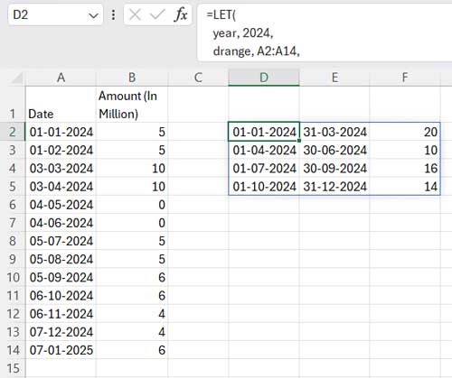
=LET(
   year, 2024,
   drange, A2:A14,
   srange, B2:B14,
   start,
      EDATE(DATE(year, 1, 1), SEQUENCE(4, 1, 0, 3)),
   end,
      EDATE(DATE(year, 1, 1), SEQUENCE(4, 1, 3, 3))-1,
   HSTACK(
      start,
      end,
      MAP(start, end, LAMBDA(s, e, SUMIFS(srange, drange, ">="&s, drange, "<="&e)))
   )
)
Insert this formula in cell D2.
Select D2:E5 and click the drop-down within the Number group in the Home tab, then select Short Date.
In this formula, you need to make three changes to use it in your dataset:
- Replace 2024 with the year of your choice.
- Replace A2:A14 with the date range, and B2:B14 with the amount range.
What makes this formula special is its flexibility. You can enter the year in any cell and replace “2024” in the formula with a reference to that cell. This way, you can quickly switch between years and effortlessly obtain quarterly sums for different years.
Formula Explanation
The Excel’s Sum by Quarter dynamic array formula employs the LET function to assign names to values or value expressions, enhancing the formula’s readability. Additionally, it improves performance by preventing repeated calculations.
Syntax:
=LET(name1, name_value1, name2, name_value2, name3, name_value3, name4, name_value4, name5, name_value5, calculation)Where:
name1is ‘year’ andname_value1is ‘2024’: Represents the year for which we want to obtain the sum by quarter of the cash flow amounts.name2is ‘drange’ andname_value2is A2:A14: Denotes the date range to summarize by quarter.name3is ‘srange’ andname_value3is B2:B14: Represents the amount to sum by quarter.name4is ‘start’ andname_value4isEDATE(DATE(year, 1, 1), SEQUENCE(4, 1, 0, 3)): Generates a sequence of each quarter’s starting dates.name5is ‘end’ andname_value5isEDATE(DATE(year, 1, 1), SEQUENCE(4, 1, 3, 3))-1: Generates a sequence of each quarter’s ending dates.
Sum by Quarter Calculation (utilizing the assigned names and values):
HSTACK(
start,
end,
MAP(start, end, LAMBDA(s, e, SUMIFS(srange, drange, ">="&s, drange, "<="&e)))
)
The critical aspect of this calculation is the following SUMIFS formula:
SUMIFS(srange, drange, ">="&s, drange, "<="&e)Where:
sum_range: srangecriteria_range1: drangecriterion1: “>=”&s (the first value in the ‘start’ date)criteria_range2: drangecriterion2: “<=”&e (the first value in the ‘end’ date)
The MAP formula iterates over each value in the start and end range, producing the quarterly sum.
The HSTACK function combines the start and end dates of the quarters with the quarterly sum calculated using the MAP function.
Sum by Quarter: Custom Function in Excel
We can transform the aforementioned dynamic array formula into a reusable function within a workbook in Excel.
The function syntax is as follows:
SUM_BY_QTR(year, drange, srange)Where:
year: Represents the year for the quarterly report.drange: Denotes the date range in the table.srange: Represents the sum range (amount column range) in the table.
Steps:
To accomplish this, we utilize the LAMBDA function in the following syntax:
=LAMBDA(parameter1, parameter2, parameter3, calculation)Let’s specify ‘year’ as parameter1, ‘drange’ as parameter2, and ‘srange’ as parameter3. The calculation will be the sum-by-quarter dynamic array formula. However, in that, you should remove the year, 2024, drange, A2:A14, srange, B2:B14, part from the beginning of the LET formula. Here it is:
=LAMBDA(year, drange, srange, LET(
   start,
      EDATE(DATE(year, 1, 1), SEQUENCE(4, 1, 0, 3)),
   end,
      EDATE(DATE(year, 1, 1), SEQUENCE(4, 1, 3, 3))-1,
   HSTACK(
      start,
      end,
      MAP(start, end, LAMBDA(s,e, SUMIFS(srange, drange, ">="&s, drange, "<="&e)))
   )
))
To create the custom function, copy this formula and open the workbook in which you want to use it.
- Go to the Formulas tab.
- Click Name Manager within the Defined Names group.
- In the Name Manager dialog box, click New.
- Type the name SUM_BY_QTR in the Name field.
- Select Workbook within the Scope field.
- In the Refer to field, replace the existing reference with the copied formula.
- Click OK and Close the Name Manager dialog box.
You are now set to use the SUM_BY_QTR() named function in that Excel workbook.
Example:
=SUM_BY_QTR(2024, A2:A14, B2:B14)Don’t forget to format the first and second columns of the result to the Short Date.


