VLOOKUP can search multiple keys and return a one-dimensional array in Excel versions that support dynamic arrays. But what about a 2D array?
For instance, imagine you need to search for 3 products in one column and retrieve available stocks and warehouse addresses. If all criteria match, you’d expect a result of 3 rows by 2 columns.
Unfortunately, Excel’s VLOOKUP with dynamic arrays doesn’t provide this feature. While it supports retrieving values based on multiple criteria from one column, it isn’t designed to return results in a structured 2D array format, spanning two or more columns. Handling 2D arrays for such tasks requires a different approach altogether.
However, fear not! I’ve devised a workaround to address this limitation with Excel VLOOKUP, and it’s surprisingly straightforward.
Sample Data, Lookup Values, and Expected Results
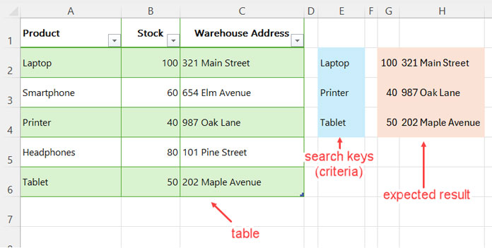
Our sample data, shown below, is spread across the range A1:C6 in an Excel spreadsheet:
| Product | Stock | Warehouse Address |
| Laptop | 100 | 321 Main Street |
| Smartphone | 60 | 654 Elm Avenue |
| Printer | 40 | 987 Oak Lane |
| Headphones | 80 | 101 Pine Street |
| Tablet | 50 | 202 Maple Avenue |
We need to look up the keys “Laptop”, “Printer”, and “Tablet” in the Product column, i.e., the range A2:C6, and retrieve their quantities and warehouse addresses from columns B and C. Here is the expected output:
| 100 | 321 Main Street |
| 40 | 987 Oak Lane |
| 50 | 202 Maple Avenue |
In short, we need to use the Excel VLOOKUP function with multiple criteria and return a two-dimensional array result.
VLOOKUP Power-Up: Multi-Criteria & 2D Array Output (Dynamic Array)
Before we delve into the formula, let’s review the VLOOKUP syntax in Excel. This will aid in understanding each parameter used in the formula:
VLOOKUP(lookup_value, table_array, col_index_num, [range_lookup])Now, let’s apply the formula to the example above to perform a VLOOKUP for multiple search keys in Excel and return a result in multiple rows and columns (a two-dimensional array).
We assume the criteria are in cells E2:E4.
Formula (in cell G2):
=LET(
     r, VLOOKUP(E2:E4, HSTACK(A2:A6, B2:B6&"|"&C2:C6), 2, FALSE), d, "|", n, 2,
     split,
          TEXTBEFORE(TEXTAFTER(d&r&d, d, SEQUENCE(1, n)), d, 1),
     IFERROR(IFERROR(split*1, split),"")
)
How to Use This Formula:
In this formula, you’ll need to make changes to the yellow-highlighted part (VLOOKUP) and the green-highlighted part to adapt it to your Excel table range.
Yellow Highlighted (VLOOKUP) Part:
lookup_value: E2:E4 (the values you want to look up)table_array:HSTACK(A2:A6, B2:B6&"|"&C2:C6)(The range of cells in which the VLOOKUP will search for thelookup_valueand the return value.)
This requires a detailed explanation. We’ve horizontally stacked the column to search for the key with the output columns combined. We want to look up multiple search keys in A2:A6 and return results from B2:B6 and C2:C6. We combined the result columns since the formula doesn’t support 2D results.col_index_num: 2 (the result column number in thetable_array)
The first column is the lookup column, and we want the result from the second column, which contains the combined values.range_lookup: FALSE (exact match of the search keys)
Green Highlighted Part:
- This specifies the number of result columns (B2:B6 and C2:C6), which is 2 in our example.
You only need to change the specified parts above to return 2D array results in Excel VLOOKUP.
Formula Logic: Excel VLOOKUP with Multiple Search Keys and 2D Array Results
The VLOOKUP function in Excel versions that supports dynamic arrays typically returns a one-dimensional array result. For instance, using VLOOKUP alone, like so: =VLOOKUP(E2:E4, HSTACK(A2:A6, B2:B6&"|"&C2:C6), 2, FALSE), would yield the following result:
| 100|321 Main Street |
| 40|987 Oak Lane |
| 50|202 Maple Avenue |
Since we used a pipe delimiter to combine columns in the VLOOKUP, we need to split the result based on this delimiter to achieve a two-dimensional array.
Although Excel provides a TEXTSPLIT function, it isn’t suitable for our case. Therefore, we’ll use a custom formula to accomplish this task.
Previously, we crafted a custom formula to split text into columns in Excel, which you can refer to here: Split Text to Columns Using a Formula in Excel (Dynamic Array). Here’s that formula for your quick reference:
=LET(
     r, A1:A6, d, ", ", n, 4,
     split,
          TEXTBEFORE(TEXTAFTER(d&r&d, d, SEQUENCE(1, n)), d, 1),
     IFERROR(IFERROR(split*1, split),"")
)
Simply replace the range to split (highlighted in yellow) in this formula with the VLOOKUP formula and the green-highlighted number, which represents the maximum number of columns in the split output, with 2, and voila!
Advantages of Using HSTACK in VLOOKUP table_array in Excel
In our VLOOKUP formula, the table_array is HSTACK(A2:A6, B2:B6&"|"&C2:C6).
We used the HSTACK function to create an array that contains the search key column as the first column and the rest of the columns (result columns) combined.
In addition to being useful for making VLOOKUP return multiple rows and columns results, it can help you solve one of Excel’s age-old problems.
That’s looking up to the left of the search key in your Excel table. Since we manipulate the range using HSTACK, we can use any column in our table as the lookup column.


