For calculating a running balance, we can utilize the SCAN function, which is a dynamic array function available in Excel.

Before we proceed, it’s important to note that dynamic array formulas are not supported in all versions of Excel. I have tested the running balance formula exclusively in Microsoft 365.

The running balance, also known as the cumulative balance, represents the net balance after considering each debit and credit transaction. It is recorded row by row, corresponding to each transaction. Examining the final value in the running balance column provides the total funds available in your account.

When maintaining separate columns for debit (withdrawals or expenses) and credit (deposits or income) transactions and aiming to compute the running balance in a third column, employing a dynamic array formula in Excel is advisable.

Sample Data in Excel Spreadsheet

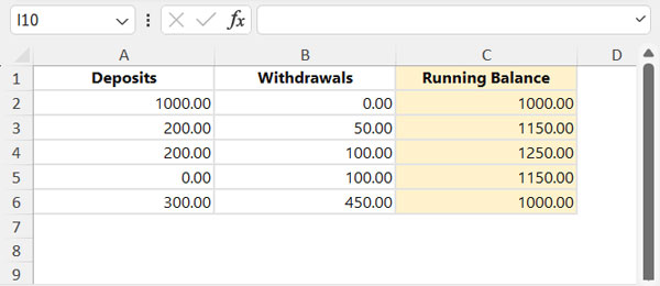
In one of my Excel spreadsheets, I have withdrawals in column A and deposits in column B. In column C, I want the running balance.

Once the formula is applied, the table should look like this:

Dynamic Array Formula for Running Balance in Excel

In the above example, I’ve used the following dynamic array formula in cell C2:

=LET(
   income, A2:A6,  
   expense,  B2:B6,  
   SCAN(0, income-expense, LAMBDA(a,v, a+v))
)

When you use this formula in your Excel spreadsheet, replace A2:A6 with the range containing your income/deposits and B2:B6 with the range containing your withdrawals/expenses.

Note:

1. The ranges must be of equal size.
2. The formula won’t work if your range references are part of a table. It will return a #SPILL error. In that case, go to any cell in the table, right-click to open the context menu, and click on Table > Convert to Range. Click Yes when Excel asks for confirmation. Alternatively, use the formula in a column outside the table range.

How does this dynamic array formula return the running balance in Excel? Let’s proceed to the formula explanation.

Formula Explanation

In the running balance dynamic array formula, we utilize the LET function to streamline it.

Syntax of the LET function in Excel:

LET(name1, name_value1, [name2, name_value2], [name3, name_value3], …, calculation)

The LET function is employed to assign names to ranges and use those names instead of ranges in the subsequent calculation.

We designate the range A2:A6 (name_value1) as “income” (name1) and B2:B6 (name_value2) as “expense” (name2).

The calculation involves the SCAN dynamic array function, which is as follows: SCAN(0, income - expense, LAMBDA(a, v, a + v))

The Calculation Aspect of LET: An Explanation of the Running Balance Formula

The SCAN function accepts three arguments. Refer to the syntax below:

SCAN Function Syntax in Excel:

SCAN([initial_value], array, lambda_function)

where:

• initial_value: 0
• array: income – expense
• lambda_function: LAMBDA(a, v, a + v)

In the lambda function, “a” denotes the accumulator, which initializes to 0, and “v” represents each element in the array.

The SCAN function applies the lambda function (a + v) to each element in the “income – expense” array, accumulating the results as it iterates. It yields the intermediate value in each iteration, forming an array of accumulated sums where each element signifies the cumulative income minus expenses up to that point.

Additional Tip: Creating a Running Balance in Growing Data with Excel

One issue with Excel spreadsheets is that they do not support infinite references from a particular row to the end. For example, if your range in the above formula is A2:A and B2:B, it won’t work. Excel requires you to specify the entire range upfront. This becomes particularly problematic with the introduction of Dynamic Array Formulas.

If your data is growing and you want your formula to accommodate those new rows in the running balance, you can make the following changes to the formula:

• Replace A2:A with INDIRECT("A2:A"&XMATCH(TRUE, B:B<>"", 0, -1))
• Replace B2:B with INDIRECT("B2:B"&XMATCH(TRUE, B:B<>"", 0, -1))

These changes will expand the dynamic running balance array formula until column B’s last non-blank row.

Resources: Excel Dynamic Array Formulas

Similar to the running balance formula, here are more tutorials covering dynamic array formulas. However, please note that they will only work in supported versions of Excel.

1. Running Count of Occurrences in Excel (Includes Dynamic Array)
2. Flip a Table Vertically in Excel (Includes Dynamic Array Formula)
3. Unpivot Excel Data Fast: Power Query & Dynamic Array Formula
4. Split Text to Columns Using a Formula in Excel (Dynamic Array)