We can utilize a dynamic array formula to split text into columns instead of using the Text to Columns Wizard in the Data menu in Excel. This helps to keep your delimited strings unaffected.
Excel offers a dedicated function called TEXTSPLIT for splitting text into columns and rows. However, it has a drawback: it cannot be applied to each row in a column without dragging it down.
Of course, you can use the REDUCE function to expand the TEXTSPLIT to each row in the range. But it’s a lambda helper function, and I don’t recommend it for very large datasets.
There is one more workaround. It utilizes the TEXTSPLIT feature for splitting by both row and column delimiters. However, this requires combining all texts in the column and placing a different delimiter to separate each row. This can also cause performance problems.
Instead of resorting to these workarounds, we can adopt a different approach to split text into columns in each row within a range in Excel. This approach involves using the TEXTAFTER and TEXTBEFORE functions.
Sample Data (Text Delimited by Commas)
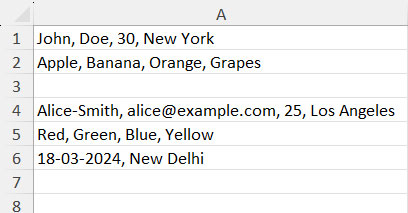
In one of the Excel spreadsheets, I have the following sample data in cell range A1:A6.
When using the dynamic array formula to split text into columns in Excel, it’s crucial to specify the delimiter correctly.
For example, the string in cell A2 is “Apple, Banana, Orange, Grapes”. You can see that the comma is the delimiter. However, it’s important to note that there is a space following each comma. Therefore, the real delimiter is not just a comma, but a comma followed by a space.
Please keep this in mind when using the dynamic array formula to split text into columns in Excel.
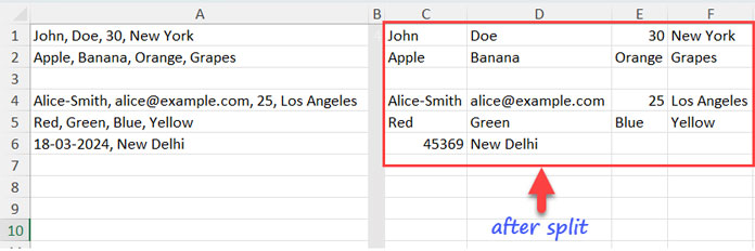
Expected Output:
Key Points:
The dynamic array formula converts numeric and date values to numbers, and all remaining values to text.
If you desire, you can make a slight adjustment to the formula to return all values as text. In this case, when utilizing numbers or dates in calculations, it’s recommended to use the VALUE function alongside it.
For example:
=VALUE(E1)The formula won’t treat consecutive delimiters as one.
For example:
- “Apple,, Banana, Orange, Grapes” will return “Apple, | Banana | Orange | Grapes”
- “Apple, , Banana, Orange, Grapes” will return “Apple | | Banana | Orange | Grapes”
If there is a blank row in the range, the formula keeps it.
Split Text to Columns Using a Dynamic Array Formula in Excel
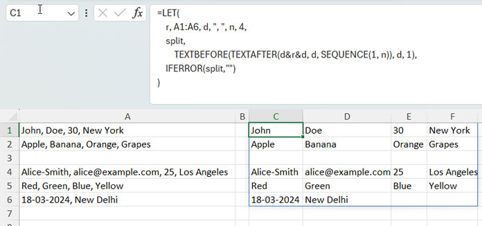
Here is the dynamic array formula to split text into columns in Excel.
=LET(
     r, A1:A6, d, ", ", n, 4,
     split,
          TEXTBEFORE(TEXTAFTER(d&r&d, d, SEQUENCE(1, n)), d, 1),
     IFERROR(IFERROR(split*1, split),"")
)
When you use this formula, replace:
A1:A6(defined asr) with the range to split.", "(defined asd) with the delimiter to split.4(defined asn) with the maximum number of columns you want in the result. In this case, you can use=LET(r, A1:A6, MAX(LEN(r)-LEN(SUBSTITUTE(r, ",", ""))+1))in any cell and refer to that cell instead of 4. The formula calculates the maximum number of items separated by commas in cells A1 to A6 (the delimiter here is “,” not “, “).
Note: If you do not wish to convert dates and numeric values to numbers, replace IFERROR(IFERROR(split*1, split),"") with IFERROR(split,"").
Formula Explanation: How the Formula Splits Texts in Each Row into Columns
Here are the step-by-step instructions for the dynamic array formula that splits texts into columns in Excel.
Extracting Text After a Given Instance of the Delimiter:
=TEXTAFTER(", "&A1&", ", ", ", SEQUENCE(1, 4))This formula follows the syntax: TEXTAFTER(text, delimiter, [instance_num], [match_mode], [match_end], [if_not_found])
Where:
text:", "&A1&", "(the delimiter is added on both sides of the text)delimiter:", "instance_num:SEQUENCE(1, 4)returns the array{1, 2, 3, 4}(it represents the number of columns in the result)
The formula extracts the text after the specific instance of the delimiter. Since the delimiter corresponds to the sequence numbers 1 to 4, it returns the following values:
| John, Doe, 30, New York, | Doe, 30, New York, | 30, New York, | New York, |
Extracting Text Before a Given Instance of the Delimiter:
By wrapping the above formula with TEXTBEFORE, we can extract the text before the first delimiter.
=TEXTBEFORE(TEXTAFTER(", "&A1&", ", ", ", SEQUENCE(1, 4), 1, 1), ", ", 1)This follows the syntax: TEXTBEFORE(text, delimiter, [instance_num], [match_mode], [match_end], [if_not_found])
Where:
text:TEXTAFTER(", "&A1&", ", ", ", SEQUENCE(1, 4), 1, 1)delimiter:", "instance_num:1
It extracts the text that occurs before a specific instance of the delimiter. Here it’s 1.
This formula eventually splits the texts in a single row into columns.
| John | Doe | 30 | New York |
To apply it to each row, replace the cell reference A1 with the range reference A1:A6:
=TEXTBEFORE(TEXTAFTER(", "&A1:A6&", ", ", ", SEQUENCE(1, 4), 1, 1), ", ", 1)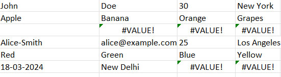
Applying LET to Clean the Split Text to Columns Formula:
We then use LET to clean the formula as per the syntax: LET(name1, name_value1, [calculation_or_name2], [name_value2, …])
=LET(
r, A1:A6, d, ", ", n, 4,
TEXTBEFORE(TEXTAFTER(d&r&d, d, SEQUENCE(1, n)), d, 1)
)
We have assigned the name r to A1:A6 (text), d to the delimiter “, ” (delimiter), and n to 4 (instance_num).
Converting Numeric Values and Dates to Numbers in Text Split to Columns:
In our final formula, we named the above formula expression, which is TEXTBEFORE(TEXTAFTER(d&r&d, d, SEQUENCE(1, n)), d, 1), with the name split.
The formula expression in the final formula is:
IFERROR(IFERROR(split*1, split),"")Where:
IFERROR(split*1, split): This part of the formula attempts to convert the text result to numbers. If successful, it returns the result as numbers; otherwise, it returns the original text. This effectively converts numbers and dates formatted as text in the result to numbers while retaining text.- The outer IFERROR function removes all other errors in the split text-to-column output.


