If you use drop-down criteria in the FILTER function, you might want to include a ‘Select All’ option to optionally exclude any specific column from the filtering criteria.
For example, imagine you have three columns and three drop-downs corresponding to them.
From the drop-down menus, you can either select a specific value or the “All” option.
- If you choose a specific value, the
FILTERfunction will filter for that value in that column. - If you choose “All,” the filter excludes that column from the filtering condition.
If you select “All” in all three drop-downs, the formula will return the data as-is, without any filtering.
Here’s how you can filter multiple columns with “Select All” drop-downs in Google Sheets:
Step 1: Set Up the Data
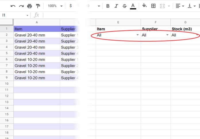
Suppose you have the following sample data in A1:C:
| Item | Supplier | Stock (m3) |
| Gravel 20-40 mm | Supplier 1 | 1000 |
| Gravel 20-40 mm | Supplier 2 | 1000 |
| Gravel 20-40 mm | Supplier 3 | 1000 |
| Gravel 20-40 mm | Supplier 4 | 2500 |
| Gravel 10-20 mm | Supplier 1 | 2500 |
| Gravel 10-20 mm | Supplier 2 | 1000 |
| Gravel 10-20 mm | Supplier 3 | 400 |
| Gravel 10-20 mm | Supplier 4 | 1000 |
Step 2: Create Drop-Downs with “All” Options
Based on the sample data, you need three drop-down menus for columns A, B, and C — each containing:
- All the unique values from that column
- An additional “All” option
We’ll create the drop-downs in E2, F2, and G2.
To create a drop-down manually:
- Navigate to cell E2.
- Click Insert > Drop-down.
- Manually enter all the unique values from column A.
- Add “All” as an extra option.
- Click Done.
Repeat this process for F2 and G2 (for columns B and C).
Tip: If you prefer to create the drop-downs dynamically from a range (including an “All” option), follow this guide: Google Sheets: Add an ‘All’ Option to a Drop-down from Range
Step 3: Apply the Formula to Filter Multiple Columns with ‘Select All’ Drop-Downs
In cell E4, insert the following formula:
=FILTER(A2:C,
    IF(E2="All", ROW(A2:A), A2:A=E2),
    IF(F2="All", ROW(B2:B), B2:B=F2),
    IF(G2="All", ROW(C2:C), C2:C=G2)
)
How Does This Formula Work?
Normally, if you were just filtering based on direct matches, you’d use something like:
=FILTER(A2:C, A2:A=E2, B2:B=F2, C2:C=G2)However, when using “All” in the drop-downs, we need the formula to ignore that column’s filter if “All” is selected.
Here’s the trick:
Each IF statement checks if the corresponding drop-down value is “All”.
For example:
IF(E2="All", ROW(A2:A), A2:A=E2)- If E2 = “All”, the condition becomes
ROW(A2:A)— meaning all rows are included. - Otherwise, it checks if
A2:A = E2.
Is ROW(A2:A) a valid filter condition?
Yes! It returns a number for each row, which is treated as TRUE in logical tests — just like LEN(A2:A), but without ignoring empty cells.
| Condition | Meaning |
| ROW(A2:A) | Includes all rows (even blanks) |
| LEN(A2:A) | Includes only rows with non-blank cells |
Tip: If you want to select all but exclude blank cells, you can replace ROW(A2:A) with LEN(A2:A) instead.
Example Walkthrough:
- In E2, select “Gravel 10-20 mm”
- In F2, select “Supplier 2”
- In G2, select 1000
The formula will return all rows matching these selections.
If you select “All” in any of the drop-downs, that column will be excluded from filtering.
Example Sheet
Conclusion
That’s it! Now you know how to filter multiple columns with ‘Select All’ options in Google Sheets using a smart FILTER formula.
Enjoy building dynamic, user-friendly filters!


