View Content from Any Sheet with Google Sheets Dropdowns

You can view content from any sheet without leaving the current sheet in a multi-sheet Google Sheets file. We will achieve this using a dropdown menu that contains sheet names.

This involves creating a dropdown menu using data validation and the INDIRECT function.

Alternatively, if you prefer another method, you can create a table of contents with clickable links within Google Sheets. This method eases navigation but does not provide an alternative way to view content from other sheets in the current sheet.

I have a Google Sheets file that contains multiple sheets with the tab names: “Home”, “Company A”, “Company B”, “Company C”, “Company D”, and “Company E”.

On the “Home” sheet, there is a dropdown menu in cell A1 containing the names of the other five sheets.

When you select any sheet name from this menu, the data from that sheet will populate starting from column B onwards.

View content from other sheets in the current sheet in Google Sheets

Sample Sheet

It’s straightforward to display data from other sheets in the current sheet as described above. Here are the step-by-step instructions:

Here’s a simplified approach to creating dropdowns with sheet names in Google Sheets without ‘directly’ using Data > Data validation: You can convert existing text to dropdowns. Let me explain how.

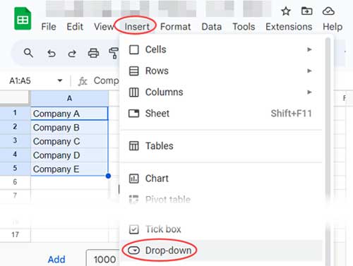
In any sheet other than the ones from which you want to display content, enter the sheet names you want in the dropdown menu. In our example, we will enter the names “Company A”, “Company B”, “Company C”, “Company D”, and “Company E” into cells A1:A5 on the “Home” sheet.

Select A1:A5, the cell range containing the sheet names, and click Insert > Drop-down. This will insert dropdown menus in A1:A5 with pre-filled sheet names as the menu items.

Quickly insert a dropdown menu in Google Sheets

Since we only need the dropdown in cell A1, let’s delete the other dropdowns in the range A2:A5. Select the cell range A2:A5 and press the “Delete” key on your keyboard.

Next, click Insert > Dropdown and choose the “Remove validation” option in the Data Validation Rules panel.

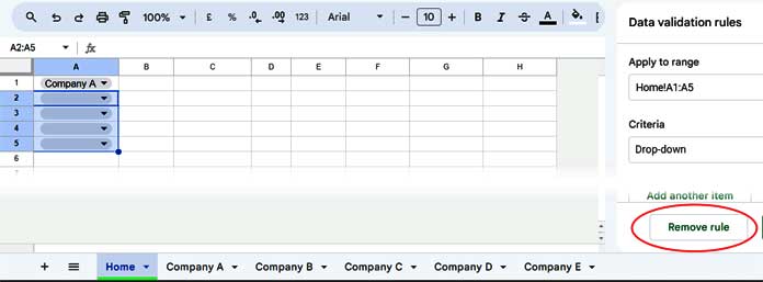
Removing multiple dropdowns quickly in Google Sheets

This will leave just one dropdown menu in cell A1 that we can use to display data from other sheets.

Step 2: Formula to Display Data from Other Sheets in the Current Sheet

We can utilize the INDIRECT function to return a cell or range reference specified by a string. This feature allows us to display content from the five other sheets in the Home sheet.

Currently, we have a sheet name selected in cell A1, which is “Company A”. We need to create a range reference like ‘Company A’!A1:Z based on it.

To achieve this, concatenate “!A1:Z” with the sheet name in cell A1 using the formula =A1&"!A1:Z".

You can use the following formula in cell B1:

=INDIRECT(A1&"!A1:Z")

When you select a sheet name from cell A1, the content from cells A1 to Z in that sheet will be displayed.

This is the easiest way to view content from any sheet using a dropdown menu in Google Sheets.

Resources

Above, we have seen how to display all contents from any sheet within the current sheet. We can also use dropdowns to control data output. Here are a few resources:

37 COMMENTS

sebastian November 15, 2023 At 12:49 am

I have followed your instructions, but I’m encountering an error: “Function INDIRECT parameter 1 value is ‘Week 1 Nov 15-16Company5’. It is not a valid cell/range reference.”

It works well until I attempt to change names in the “Sheet Names” tab.

- Prashanth KV November 15, 2023 At 8:20 am
  
  Hi Sebastian,
  
  In the “Sheet Names” tab, replace “Week 1 Nov 15-16” with “Week 1 Nov 15-16!”.
  
  Note the leading exclamation mark. Once you’ve made this change, select the new name from the drop-down. That should resolve the issue.
  
Jeffrey Smith March 14, 2022 At 6:17 am

I have followed every step of this without issue.

However, when I use the Master Tab and select the desired item on the drop-down, it is only pulling up the correct named range for one of them.

When I select a different name on the drop-down, it populates the wrong data.

- Prashanth March 16, 2022 At 2:12 pm
  
  Hi, Jeffrey Smith,
  
  Please check the named ranges.
  
  Also, you can share the URL here, which I won’t publish for me to check.
  
  - Jeffrey Smith March 17, 2022 At 4:02 pm
    
    I have redone the named ranges a few times, and it does the same thing. Hoping you can find my error.
    — sample sheet URL removed by admin —
    
    - Prashanth March 18, 2022 At 10:50 am
      
      Hi, Jeffrey Smith,
      
      Sorry! The issue was with my formula.
      
      I haven’t specified the is_sorted optional argument in my formula.
      
      VLOOKUP(search_key, range, index, [is_sorted])
      
      We must specify it to FALSE or 0 (zero) and I have edited my post.
      
      So use the below Vlookup formula
      
      =VLOOKUP(A1,'Sheet Names'!A1:B14,2,0)
      
      You can optionally use IFNA with INDIRECT since your datasets in each tab contain #N/A!
      
      =ifna(INDIRECT(A1&B1))
      
Luke October 13, 2021 At 2:04 pm

Hi,

Can you please make a video of this?

I keep getting an error with the indirect function.

I want to be able to edit or add information on the master sheet instead of having to open each sheet when I want to add data.

- Prashanth October 14, 2021 At 2:14 pm
  
  Hi, Luke,
  
  If you share the sheet (sample), I may be able to sort out the error.
  
  The formula won’t permit you to add information to the master sheet. That’s a drawback.
  
jon October 14, 2019 At 7:46 am

Shared again.

Thank you.

- Prashanth October 14, 2019 At 1:34 pm
  
  Hi, Jon,
  
  The issue is due to mixed content in the column. For example, column 6 (TRAIN column) contains numbers in some tabs, text in some other tabs. The query will treat the majority values in such columns as the column type. So you will see the wrong outputs in Query filtering.
  
  You can solve this issue by converting the value type which I have detailed here.
  
  How to Solve the Mixed Data Type Issue in Query in Google Sheets.
  
  Best,
  
jon October 11, 2019 At 6:37 am

Hi,

Already shared in view mode.

Also if I delete data in column train for the month of June to Dec. Data in the Search_Train tab will go blank.

Thank you.

- Prashanth October 11, 2019 At 11:04 am
  
  Hi, Jon,
  
  I’ve accidentally deleted that mail. Share again, please.
  
  Best
  
jon October 10, 2019 At 2:34 pm

Hi,

I already made one for my project.

I encountered an error when I entered a date in the month of June, the “search_Train” tab will go blank.
I cannot figure out the error.

Could you please look into the error.

I appreciate your help and thank you very much.

Jon

- Prashanth October 10, 2019 At 6:31 pm
  
  Hi, Jon,
  
  Happy to help you if you can share your Sheet in View mode.
  
  Best,
  
jon October 9, 2019 At 10:10 am

Thank you very much, Mr. Prashanth.

jon September 19, 2019 At 12:14 pm

Hi Prashanth,

Can I search like, I have 31 sheets as in for 31 working days, (sheet named day1 up to day31)

On sheet day1, data is Name / Transactions / Amount.

How can I search Mr. A’s transactions from Day 1 to Day 31?

Thank you.

- Prashanth September 19, 2019 At 1:01 pm
  
  Hi, Jon,
  
  I couldn’t access your Sheet! Sent a request.
  
- Prashanth September 20, 2019 At 1:20 pm
  
  Hi, Jon,
  
  Name the range (Data menu > Named ranges) in each tab like Day_1, Day_2 …
  
  Then use that in Query.
  
  =Query(ArrayFormula({Day_1;Day_2}),"Select * where Col6='"&A2&"'",1)
  
  You can find this formula in cell B2 in the Master tab of this Sheet. I have only added two named ranges.
  
  You can expand it like;
  
  {Day_1;Day_2,Day_3;Day_4}
  
  If you are adding tabs each day, then you can include that future tabs too in the formula. In that case, you may find the following tutorial useful.
  
  How to Include Future Sheets in Formulas in Sheets
  
  Best,
  
Ian September 9, 2019 At 9:03 pm

Attached is a link to a mockup of the sheet I am working on! Thank you for your help!

— Link removed after copying —

- Prashanth September 10, 2019 At 10:19 am
  
  Hi, Ian,
  
  See my attempt on the Master tab.
  
  Practice Burden Calculator
  
Ian September 7, 2019 At 2:08 am

Hi Prashanth,

This is great info! I am trying to add data validation drop down lists to each of the “company” tabs and they don’t seem to transition well to the master sheet.

I also have multiple charts on each tab and it only seems to pull one charts from each of the “company” Tabs.

If you have any recommendations or wouldn’t mind taking a look at my sheet it would be greatly appreciated! Thanks.

- Prashanth September 7, 2019 At 10:57 am
  
  Hi, Ian,
  
  No issue! you can share (copy of) your Sheet with me. I just prefer a Sheet copy with some mockup data.
  
  Best,
  
Shawn August 25, 2019 At 4:51 pm

Hi,

Thank you for this! I’m trying to do the same thing for a grade book I use for my class (instead of pulling and viewing data, I’d like to edit and add data) but I can barely pull and view the data. I see N/A as soon as I do the Vlookup function. What do you recommend? Thanks.

Bowski March 7, 2019 At 7:28 pm

Hi Prasanth,

I tried to do this on the LibreOffice but when it comes to the indirect function it is showing #ref.
I tried to download your sample and opened on libre office and same error pops out. I’m not sure if there is any indirect function we can use on LibreOffice.

- Prashanth March 8, 2019 At 11:09 am
  
  Hi, Bowski,
  
  I am not familiar with LibreOffice. The Indirect function is different in Excel and Google Sheets too.
  
  Comparison: Indirect in Excel vs. Indirect in Google Sheets
  
  So there may or maynot be some changes in the use of this function in LibreOffice. Please check their support page HERE.
  
Ben T. Lador October 2, 2018 At 12:16 pm

Hello,

I got an error upon applying the “Indirect function” saying that my named range is not a valid cell/range reference, but I follow all the steps in the tutorial. Is there anything I have missed?

- Prashanth October 2, 2018 At 3:03 pm
  
  Hi, Ben T. Lador,
  
  I can’t say what’s the actual issue.
  
  Better please do check my example sheet. I have already shared that with a previous commenter. Please go through the comments and follow the demo sheet link.
  
Horse September 19, 2018 At 10:40 am

Hi, I’m a newbie to excel and google sheet, I got an interesting idea after reading your post:

We can just PULL and VIEW data from other sheets in the MASTER sheet,
but we can’t EDIT or ADD data in the MASTER sheet.
By expanding the range of every name range, I mean, like changing “CompanyA!A1:E10” to “CompanyA!A1:E999”, we get the blank cells of the original sheet in MASTER, if we can make changes in the MASTER sheet, that would be awesome.

Is this idea vagarious or there is some formula we can do this?

Thank you for your sharing!

- Prashanth September 19, 2018 At 11:36 am
  
  Hi,
  
  That’s doable.
  
  Please do the changes as follows.
  
  1. CHANGES IN THE TAB ‘Sheet Names’
  
  In the tab “Sheet Names” in cell B2 enter the below formula.
  
  ="A1:"&left(address(1,counta('Company A'!A1:1),4))
  
  In cell B3, copy the same formula but change the sheet name, i.e. ‘Company A’ to ‘Company B’
  
  Repeat this for other sheets. That means instead of named range, we are going to use cell reference.
  
  2. CHANGES IN THE TAB ‘Master’
  
  Replace the Indirect formula in Cell C2 with the below one.
  
  =query({indirect(A2&B2)},"Select * where Col1 is not null")
  
  Hope this helps.
  
  - Obed Gaytan November 12, 2020 At 2:12 am
    
    I attempted to do this on my sheet, but I couldn’t get it to work properly. It would be nice to be able to use this to pull information without having to create Named ranges for every sheet.
    
    Is it also possible to also edit information in the master sheet pulled from the other sheets?
    
    - Prashanth November 13, 2020 At 2:39 pm
      
      Hi, Obed Gaytan,
      
      We can pull information from other sheets without creating named ranges. If you share your sheet (just a demo sheet), I would try to help you out.
      Regarding your second question, we can’t edit the pulled data. If we edit, the formula would break.
      
Nicholas A Stockbridge September 18, 2018 At 6:35 am

I got it to start pulling but the sheet is only pulling Monday for Monday and Sunday
And pulling Sunday for Tuesday-Saturday. I dont get what is wrong :/ Ive double checked all names Ive retyped names.

- Prashanth September 18, 2018 At 10:22 am
  
  Hi, Nicholas,
  
  Can I have a view of your sheet?
  
Ben February 22, 2018 At 10:59 pm

The formulas contain a parcing error when I duplicate your efforts. Would you please share this with me? THanks!

- Ben February 22, 2018 At 11:08 pm
  
  Just Kidding, I found the reference error. Is there a way to make the formatting of the data range transfer from the source to the ‘master’ page?
  
  - Prashanth February 23, 2018 At 8:56 am
    
    Hi Ben,
    As committed please see the link.
    
    https://docs.google.com/spreadsheets/d/1ouEoAoFwwaNaNqpbQ1St8lYE8mNRTestHBoqJyYw-uk/edit?usp=sharing
    
    To get the edit access, please make a copy from File menu.
    
    Prashanth 🙂
    
- Prashanth February 22, 2018 At 11:33 pm
  
  Hi Ben,
  Let me check, If available I’ll post it soon.
  Thanks.