In this tutorial, I will explain the steps to obtain only unique values in a drop-down list in Google Sheets.
What does it mean?
If an item is already selected in one drop-down, it won’t be available for selection in another drop-down. This prevents duplicates in the drop-down selections.
Removing Used Items from Data Validation Drop-Down Lists – Understanding the Scenario
Please see the illustration below.
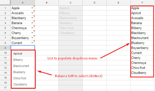
In the provided screenshot, column A contains drop-down menus that populate values from column F. As shown, I’ve already made selections in the drop-down lists from rows A1 to A8.
When I click the drop-down menu in cell A9, it only displays the values that have not been previously selected. This prevents duplicate selections. I hope this explanation clarifies the concept.
This functionality is referred to as displaying distinct values in a drop-down list in Google Sheets or removing used items from the new drop-down.
How to Get Distinct Values in a Drop-Down List in Google Sheets
The solution revolves around using a helper column.
For example, if the list to create the drop-downs is in column F, which contains three items:
| APPLE |
| ORANGE |
| MANGO |
Suppose you have selected APPLE in a drop-down in column A. In the next drop-down, you should only get the following values:
| ORANGE |
| MANGO |
So, in column C (the helper column), we will use a formula to generate a list from columns F and A with values that appear only once.
So, in short, to get distinct values in a drop-down, we need a helper column that contains unique values.
Unique values are values that appear only once in a range, and distinct values are values in a range after removing duplicates.
How is that possible?
Using a function in cell C1 (the first row in the helper column), we can get unique values.
Formula and Explanation
In cell C1, enter the below UNIQUE formula to generate unique values, which are the values that only appear once in the combined range:
=UNIQUE(VSTACK(F:F, A:A),,TRUE)The VSTACK(F:F, A:A) constructs an array by combining the ranges F:F and A:A vertically. The UNIQUE function then returns values from this array that only appear once.
Use this unique output to create drop-down lists with distinct value selections in Google Sheets.
Use Data Validation to Create Distinct Drop-Down Lists
When I mention getting distinct values in a drop-down list in Google Sheets, I’m simply referring to avoiding duplicates in the drop-down menu/list.
I’ve already generated unique values in column C. Now we need to create drop-downs in column A. Here are the steps:
Steps:
- Navigate to cell A1.
- Click on “Insert” in the menu bar, then select “Drop-down.”
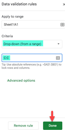
- In the criteria section of the data validation rules panel, choose “Drop-down (from a range).”
- In the field below, enter the range C:C.
- Click “Done.”
Copy the drop-down in cell A1 and paste it down as far as you need.
We’ve completed all the steps involved in generating drop-down menus that only contain distinct values.
Notes:
- Disregard the “Invalid” error indicator/marks on the drop-down item selected cells.
- If you copy and paste a filled drop-down (a drop-down with a value selected), remove the value from the pasted drop-down to avoid duplicates.
Additional Tips: Adjusting the Formula When Drop-Downs are Arranged Horizontally or in a 2D Array
Things are made very straightforward since we have functions like VSTACK and TOCOL.
Obtaining Distinct Values for Drop-Downs in a Row (Horizontally):
Assuming the original list to create the drop-downs is in column N. You want the drop-downs in cells C1:G1.
We require a helper column, let’s consider column K. In cell K1, input the following formula:
=UNIQUE(VSTACK(N:N, TOCOL(C1:G1)),,TRUE)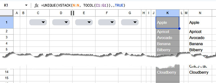
Here, N:N represents the original list range, and C1:G1 represents the drop-down range.
Create the drop-down in cell C1 using values in column K, then copy and paste into cells D1:G1.
Obtaining Distinct Values for Drop-Downs in a 2D Array:
The drop-downs are needed in cells C1:G10, and the original list is in column N. If so, input the following formula in cell K1:
=UNIQUE(VSTACK(N:N, TOCOL(C1:G10)),,TRUE)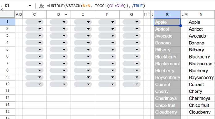
Here, N:N represents the original list range, and C1:G10 represents the data validation drop-down range. Create the data validation drop-down in cell C1 using the values in column K.


Can the Distinct Values in Google Sheets be applied to a range of cells and then to a different range of cells?
For example, I have weekly students coming, so I want their name to disappear once they have scheduled an appointment, but I want to keep the same dropdown list for next week. Is it possible?
Hi, Mord Stater,
You require to modify the formula.
Replace the range reference of the existing drop-down in the formula with the new drop-down range.
(replace
{F1:F;A1:A}with{F1:F;B1:B}) – A1:A – old drop-down, B1:B – new drop-down.Hi Prashanth
I’m always getting this error.
“Error
Array result was not expanded because it would overwrite data in xxx.”
Hi, Sathish,
All the cells below the error cell must be empty/blank.
Hi, do you like this solution? For your first example in the Text sheet:
=filter(F:F,countif(A:A,F:F)<1)Hi, Andrea G.,
That’s cool 🙂
Here is another one.
=unique({F:F;A:A;""},0,1)Hello Prashanth,
I am using your sample sheet with my test data.
Col A (Drop Down, Data Validation, Reference Col C)
Col C (Distinct Data generated from Col F) – I am getting an error here.
Col F contains data where cells have Alpha Numeric, Numeric, Text, and Symbol as data).
Thank you in advance.
Hi, AJ,
If the data contains mixed-type data (number, text, date, etc.), Query won’t return the correct result.
The good news is now we can use the UNIQUE function for the said purpose.
Filter Distinct Columns or Rows in Google Sheets – UNIQUE Improvements
So, instead of the QUERY(), you can use the below simple formula in C1.
=unique({A1:A;"";F1:F},false,true)Note:-
It seems you have shared a sample sheet. But without editable rights. Also, I could not find the mixed data type issue in your sheet.
The formulas were working quite fine there.
How can I make this work across multiple rows?
Hi, Adam,
I’ve added a new tab named “Across Rows” in my example Sheet.
You can check the last part of this tutorial for that Sheet’s link.
Hi Prashanth!
Great explanation, I’m really new to formulas but made it work using the arrayformula option. For me, instead of having a separate column of dropdowns, I have a dropdown above the referenced column. Here’s what I used:
=ARRAYFORMULA(IF(COUNTIF(A8:A,J8:J)=0,J8:J,))A8:A – not sure what this does
J8:J – contains the data
J4 – has the data validation (used to be “list of items” until your formula)
The data validation is in J4, and I put your formula in O8. Everything works well, but I also have conditional formatting for when J8:J matches J4, the background color changes to yellow. To work around all the columns turning yellow when J4 is empty, I had a default selected.
My new problem is that when J8:J is empty then J4 is empty and all the boxes turn yellow. Do you know how to make it so the background of a cell in J8:J only turns yellow when something is present in J4 and they match, but remains white when both are blank (and without errors)?
Hope this made sense… would appreciate any help I can get! Already thankful for the article.
Daniel
Hi, Daniel,
I am in the dark. Can you please make a copy of your sheet, replace the original data with some sample (mockup) data, and share that sheet URL in the reply below?
Dear Prashanth,
First of all – tremendous job, used your queries a lot of times but this time I got stuck (due to lack of abilities of course ;).
Could you please take a look at the following sheet?
… link removed by admin …
I have made a copy just for the test. What I need is to assign wedding guests (column P) to tables. I need drop-down lists on every C3:N12 field. I have spent 3 hours trying to set it up and now I am losing my mind 🙂
What I need of course is to make every guest name unique, once used in any column, cannot be used again.
Could you please advise?
BR,
Mateusz
Hi, Mateusz Szkudlarek,
I have made a copy of your example sheet and solved the problem in that.
You may please make a copy of the same from here.
Wedding Table Sample
In that sheet, you can find the following formula in cell Q2.
=filter(P2:P,regexmatch(P2:P,"^"&textjoin("$|^",true,C3:N12)&"$")=FALSE)The output of the above formula used for creating the drop-downs.
You are a god! is there any way to support you somehow?
Hi, Mateusz Szkudlarek,
Thanks for the kudos!
Thanks, this works in a column…
I need to do two dropdown lists in successive columns.. like A and B.
Column B hides selected items in column A and this rule is repeated in every row.
In other words, the same full list shows in the dropdown list in column A of the second row…
Hi, Hassan Maateeq,
Sorry! I’m in the dark. An example sheet may help me.
Thanks so much, Prashanth!
I don’t have an example sheet because I haven’t been able to work. But what I was trying to accomplish was not having a list in other cells (P2:P10).
I was hoping to just enter values into A2 and as more information is entered, a drop-down list would be built in the A column.
Hi, tomP,
Using a helper column, you can achieve that.
In cell P2, key the following FILTER formula (this column is going to be our helper column).
=ifna(filter(A1:A,A1:A<>""),"Apple")Replace “Apple” in the formula with the very first value, that you are going to enter in cell A2.
Select A2:A20 (or A2:A) and go to Data > Data validation > Criteria > List from range.
In the field against the “List from range”, Select P2:P and SAVE.
Note: You can hide the helper column P.
I would like to do the opposite in a dropdown.
I have a column titled “Requesting Unit”. It is not a completely fixed data set.
I know that sheets will suggest other entries in the row, but I would like for the list to be compiled in data validation to make it easier in the long run…less typing.
Is there a way to take each entry in the column and have it be added to a data validation list? i.e. 1st “row-RR7J”, 2nd row “RQ7T”, etc. But after each row is entered by typing, it is automatically added to a data validation list. Thanks
Hi, tomP,
Assume your list is in P2:P10 and creating drop-down in A2.
In data validation Criteria > List from range, select P2:P instead of P2:P10. So that future values will be added to the drop-down list.
Please share an example sheet, if this is not what you were aksing.
Nice work! Really helpful, I give you my thanks!
Hi There!!!
Maybe you can help me….
I applied the formula and is working perfect…. the problem is:
In my Google Sheets I have 2 columns:
1) date of appointment
2) time of appointment (dropdown with options – Morning, afternoon, evening).
The idea is the user selects a date and then checks the available slot in the dropdown…
IMPORTANT: Every time I have a new user it will be adding a new row in the sheet
The problem is how can I remove the used options in the dropdown if the user chooses the same date?
For Example:
1)User A choose January 01 – morning
2)User B choose also January 01 – but now the dropdown supposed to show only the options “afternoon” and “evening”.
3)User C choose also January 01 – now the dropdown supposes to show only the left option.
This means that every time I have the same date in the column “DATE”, the dropdown in the column “TIME” only shows the left options (options not taken already).
I will be very thankful for your help!
Thanks a lot,
Gerson.
Hi, Gerson,
We can’t do that using a formula as in Google Sheets we have limited control over the drop-down.
Hello, I was wondering the same.
How did you end up doing it then? I tried using
=query(query({'sheet'!H6:H7;P1:P2},"Select Col1...not to avail…
Any help appreciated! Thanks in advance.
Hello, Tribune,
I guess you want to keep the distinct value drop-down menu in one sheet (Sheet1) and the supporting data in another sheet (Sheet2).
Here are the changes required.
In Sheet2;
Range F1:F contains the list of items.
The Formula to use in cell C1 in that sheet.
=query(query({F1:F;Sheet1!A1:A},"Select Col1, count(Col1) where Col1<>'' group by Col1"),"Select Col1 where Col2=1")In Sheet1;
In Datavalidation select/enter the criteria range Sheet2!C:C.
Best,
Hello,
I was wondering if it is possible to have the drop-down menus on a different sheet than the selection and helper menu? How would you edit the query for this? Thank
Nevermind, I figured out the solution for this.
I would love to know how you fixed this… I have one sheet where the drop-down menu(s) will appear…and another sheet where the range lists exist (F column and C column like the example above).
But when selecting from the drop-down – the selections will not disappear.
Hi, dave2112,
In your case, the list to use is in Players!C1:C and the drop-downs you want in Pool!F4:Z12. So in data validation, follow the below settings:
Cell range: Pool!F4:Z12
Criteria > List from a range: =Players!$C:$C
I have already applied the above settings in your shared file “2021 TPC Pool – A”.
=Players!$C:$C
OMG, thank you so much! Your solution worked perfectly!
Well, I needed a little update for using numbers instead of text strings, but now it’s working perfectly!
My Helper column is listing the number values in numerical order, but my drop-down list restores my previously randomized order – which is exactly what I wanted.
So I just wanted to drop by and let you know how much I appreciate your article! So often I find fixes that are clunky workarounds or just don’t work. Your solution is rock solid! Thank you!
Just so you know, I’m creating an inventory list for equipment used in my company. The unique data that this solution helps with is registration numbers for each piece; so no duplicates are allowed.
With hundreds (and later thousands) of pieces of equipment in our inventory, you can see just how helpful/useful this solution is! Thanks again!
Ok, so I had an error in my sheets. But the only real change once fixed is that the range is not randomized per my preference. But everything still works. Would I be able to randomize the range in the generated list below the formula?
Hi, Valerie Ann Savage,
I have two different formulas to use in cell C1 (helper column).
Use the Countif formula instead of Query for keeping the order as per your original list in column F.
NB: My Query formula won’t work in a number column. It should be modified like this.
=query(query({F1:F;A1:A},"Select Col1, count(Col1) where Col1 is not null group by Col1"),"Select Col1 where Col2=1")If you want any additional help, feel free to share a copy of your Sheet or an example Sheet without any personal/confidential/sensitive data.
Best,
Hi there,
This formula is exactly what I was looking for.
Sadly it doesn’t work for me at all. It always gives me #ERROR! Even when I copy your entire sheet, that you linked above, to a new one.
I also tried to set it up from scratch. Still didn’t work even though I used the same exact same columns as you did.
When I open the sheet you linked, everything is working fine.
Is there any option I have to activate in the new sheet to make it work?
Also, in your sheet, you only have the query formula in C1. How does the formula pass the information (leftover fruits) into C2-C18?
Thanks in advance.
Hi, derSaft,
The error is probably due to the ‘Locale’ settings of your Sheet.
Solution:
Copy my Sheet and go to the menu File > Spreadsheet settings.
There change the Sheets ‘Locale’ from the United Kingdom to your country. Time Zone is not important, but you can change that too.
This will modify the existing Query formula based on the new Locale (In EU countries, the formula uses a semicolon instead of a comma).
Now you can copy the content of the Sheet to any other Sheet without error.
Now to your second question, that is;
How does the formula pass the information (leftover fruits) into C2:C18?
In the Query formula, the DATA is the values in column A and column F combined.
{F1:F;A1:A}I have used the Count aggregation function in Query to count the values in this virtual column. If the count returns the # 1, such values are distinct. I have filtered that distinct values.
Best,
Hi Prashanth,
Thanks so much for the reply!
It was indeed the switching from commas to semicolons. Now everything is working fine 🙂
I saw that you also included a version that lets you use the script for dropdowns in different columns instead of only one.
I was wondering if there’s actually a fast solution which combines both versions (multiple columns + multiple rows).
I’m using 8 columns that each have 5 rows as dropdowns (same source for all 40 dropdowns).
I guess since you use TRANSPOSE which just switches columns and rows, it’s not that simple to combine both, right?
Do you know of any workaround for this or have any other tutorials that might help?
Thanks!
Greetings from Germany
Hi, derSaft,
It’s a tough task to add multiple columns. I don’t find an immediate solution to this.
Hi,
This article is definitely helping and thanks for the effort!
However I now encounter a case that I’m going to make 2 dropdown list where both of their dropdown items are same.
When the first dropdown item is selected, the second dropdown list should exclude the selected item in the first dropdown list to prevent from same items selected twice.
Both of the dropdown list items are based on a list of items rather than a list of range…
Do you have any idea on this one?
Again, this article is really helpful for me!
Best
Hi, Ben,
You are welcome!
At present, there is no way to achieve that using data validation “List of items”, instead of “List from range”.
Best
Hello,
Thank you for your explanation.
I was wondering if it was possible to do the same with several drops down columns instead of just one big column? I tried changing the cell references with this:
=query(query({F1:F;C1:G1},"Select Col1, count(Col1) where Col1'' group by Col1"),"Select Col1 where Col2=1")but it does not work…
Thank you for your time.
Best
Hi,
It will work. But the formula won’t be like that.
There is one contradiction in your formula. Since your drop-down menus are in C1:G1, how the F1:F (master list) can contain the source. It can be F2:F, or any other column.
I am using N1:N as the source list. Then the formula will be like this.
=query(query({N1:N;transpose(C1:G1)},"Select Col1, count(Col1) where Col1<>'' group by Col1"),"Select Col1 where Col2=1")I have this formula in cell K1. Accordingly, please change the settings in the data validation rule.
I have demonstrated the same on my Sheet (See the Sheet link in one of my previous comment above)
Best
Thank you for your help!
Do you have an example spreadsheet link to share with this query in action? I am copying this setup verbatim but am unable to get the query to output the list of remaining unselected items.
Hi, billc,
Luckily I do have a copy of that Sheet which I have included in the last part of this tutorial.
Thanks.
I dont know how to get this to work with numbers instead of words(fruit)
Hi, Sean McNamara,
Replace the Query formula as below.
=query(query({F1:F;A1:A},"Select Col1, count(Col1) where Col1 is not null group by Col1"),"Select Col1 where Col2=1")Thanks.
TY