We can use custom formula rules to highlight (conditionally format) unique and distinct values in a column in Google Sheets.
Unique values are those that appear only once in a column, while distinct values are obtained after eliminating duplicates.
This terminology may be confusing because we typically refer to the output of the UNIQUE function as unique values. However, the function is capable of returning both unique and distinct values.
Syntax: UNIQUE(range, [by_column], [exactly_once])
The confusion arises from the fact that when you apply UNIQUE to a column with default settings (‘exactly_once’ set to FALSE), it returns all distinct values. However, we generally call the UNIQUE function output to unique values.
Therefore, in tutorials that do not explicitly mention the term “distinct,” we generally refer to the output of the UNIQUE function as unique values.
How to Highlight Distinct Values in Google Sheets
We will use the COUNTIF function to highlight distinct values in a column in Google Sheets.
Assuming we have data in column A starting from cell A2 up to A10 (cell range A2:A10), to highlight distinct values, use the following custom formula rule in conditional formatting:
=COUNTIF($A$2:A2,A2)=1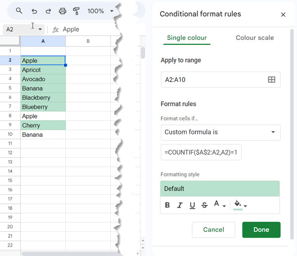
As evident, the formula only highlights the initial occurrence of values within the range.
Steps to Apply the Rule:
- To apply, select A2:A10 or from A2 up to the row you want the rule to be applied.
- Go to Format > Conditional formatting.
- Under “Format rules,” select “Custom formula is.”
- Copy and paste the above formula in the field below.
- Click Done.
Formula Explanation
The formula (highlight rule) we used in the conditional formatting to highlight distinct values is essentially a COUNTIF function.
Syntax: COUNTIF(range, criterion)
The range to count is $A$2:A2, which means from cell $A$2 to the current row (A2), and the criterion is A2, referring to the value in the current row.
So, in each row, the formula returns the count of the values in that row from the start of the range. If it is equal to 1, the formula highlights the cell.
This is an example of the effective use of absolute and relative cell references in highlighting.
How to Highlight Unique Values in Google Sheets
We can use the UNIQUE function with the parameter exactly_once set to TRUE to extract unique values in a list.
In our sample data, we can use the following formula to extract unique values:
=UNIQUE($A$2:$A$10, ,TRUE)Note: The range used in UNIQUE is $A$2:$A$10. If you refer to the entire column such as $A$2:$A, use the following formula: =TOCOL(UNIQUE($A$2:$A, ,TRUE), 1). The TOCOL wrapper removes a blank cell from the bottom of the result caused by open-range usage.
Once we have unique values, we need to match the values in the highlight range with this result. For that, we can use the XMATCH function.
Syntax: XMATCH(search_key, lookup_range, [match_mode], [search_mode])
Here is the custom formula rule to highlight truly unique values in our sample data:
=XMATCH(A2, TOCOL(UNIQUE($A$2:$A, ,TRUE), 1))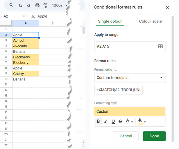
The rule matches the current row value in the list that contains truly unique values and returns its position in the list. If not found, it returns #N/A. Google Sheets highlights the cell wherever a match occurs.
You can follow the same steps outlined for highlighting distinct values to apply this highlighting rule as well.
Want to explore more?
Check out the Ultimate Guide to Conditional Formatting in Google Sheets for a complete collection of formula-based highlighting techniques.


