Creating a dynamic range in charts is straightforward in Google Sheets. But first, what is a dynamic range?
A dynamic range ensures that when new rows or columns are added to the data used for creating a chart, the chart updates automatically. Let’s explore this with examples.
When plotting a chart in Google Sheets, you need to specify a data range. For instance, suppose you created a chart using the range A1:B2. If you later add another row, expanding the range to A1:B3, the chart should automatically include this new row if it’s dynamic.
This concept applies to columns as well. If you add data to C1:C3, the chart should include those values too.
Dynamic Row Ranges in Charts in Google Sheets
Dynamic ranges for rows are supported in Google Sheets. For example, even if your data range is set to A1:B2, Google Sheets will automatically detect newly added rows and adjust the chart accordingly.
If you don’t want the chart to include new rows, simply leave a blank row after the last row containing data before adding new entries.
Dynamic Column Ranges in Charts in Google Sheets
However, the above behavior doesn’t apply to columns. Consider the following sample data in A1:K4:
| Year | China | India | USA | Indonesia | Brazil | Pakistan | Nigeria | Bangladesh | Russia | Mexico |
| 2000 | 1270 | 1053 | 283 | 212 | 176 | 138 | 123 | 131 | 146 | 103 |
| 2015 | 1376 | 1311 | 322 | 258 | 208 | 189 | 182 | 161 | 146 | 127 |
| 2030 | 1416 | 1528 | 356 | 295 | 229 | 245 | 263 | 186 | 149 | 148 |
If you add data to column L, expanding the range to A1:L4, the chart will still reference only A1:K4.
To make column ranges dynamic, you must select additional blank columns when creating the chart. Follow these steps:
- Select the range
A1:M4, including two additional blank columns (or as many columns as needed). - Click Insert > Chart.
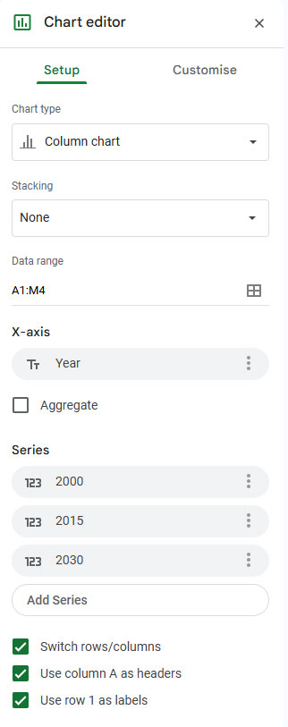
- In the Chart Editor, under the Setup tab, select “Column” or “Bar” as the chart type, as the above data is well-suited for these chart types.
- Update the data range to
A1:M4if it hasn’t been set automatically.
Creating a Chart with Dynamic Ranges from Formula Outputs
Now, let’s explore dynamic ranges generated by formulas. We’ll use the same sample data as above, located in A1:K4, which lists the top 10 most populous countries by year.
Creating a Drop-down Menu with Years
- Navigate to cell
N1. - Click Insert > Drop-down.
- Enter the values
2000,2015,2030, andAll. - Click Done.
This will create a drop-down menu with an “All” option.
Filter Formula for the Dynamic Range
In cell O1, use this formula:
=ArrayFormula(
     IF(
        N1="All",
        A1:M,
        {{A1:M1}; FILTER(A2:M, A2:A=N1)}
     )
)
Explanation:
- If “All” is selected in the drop-down, the formula returns the entire range
A1:M(actual data with two empty columns for future country data if added in columns L and M). - Otherwise, it filters rows based on the selected year while preserving headers using curly braces (
{{A1:M1};...}).
Creating the Chart
- Select the range
O1:AA15(the actual filtered data will be in O1:Y, with two empty columns reserved for potential future country data in columns Z and AA) - Go to the Insert menu and select Chart.
- Choose “Column Chart” as the chart type.
- Modify the data range to
O1:AA15.
Now, the chart dynamically adjusts as per the drop-down selection.
The above is actually an example of a dynamic row range in charts, even though we added additional columns. These columns currently do not contain any data.
Additional Tip: Filtering by Columns
Below is an example demonstrating how to visualize a dynamic column range in a chart.
To filter by columns (e.g., country names):
- Create a drop-down in
N1with all country names and an “All” option. - Use this formula in
O1:
=IF(N1="All", {A1:M}, {{A1:A}, FILTER(A1:M, A1:M1=N1)})The steps for chart creation remain the same.
Resources
We have seen examples of using dynamic ranges in charts in Google Sheets. Here are a few additional resources related to charts and filtering for charts.


Thanks for this. I was looking for this. Especially the extra Sheet3.
Prashanth,
It was a great tutorial. I may have a bit more complex of a situation where I need my data and charts to be more dynamic than they are currently.
I track dates of training completion and graph them by the department. As employees come and go, I add and delete rows of data, and I need my charts to be dynamic to respond to more or fewer employees within that department.
I could use a little extra help beyond this tutorial.
I’d be happy to allow you access to my sheet. But not sure how to do that in this setting.
I also need to maintain confidentiality with the sheet. Would you be able to help me with my situation.?
Hi, Matt,
Feel free to share the URL of the sheet below in your reply. I won’t publish that URL.
You may replace personal info like real names, phone numbers, or email IDs with dummy info.
Let’s try.
Hi Prashanth,
Great article! I am having trouble adding the Series label in the Setup tab. In your sample (Sheet3), the label is dynamic and cannot be changed. Where is that set up? If I copy past my data to your sheet is works but when I do one from the scratch I can’t do it. Also, in my case, even I manually insert the country name as a label, it does not appear as the label on the chart.
Any idea?
Many thanks
Hi, Abbas Mousavi,
I may require access to your sheet. Can you share a mock-up sheet?
Thanks for the info Prashanth. Very clever!
I would like to be able to filter up to and including values. So for your example, if I selected 2015 for the filter, I would like the filter to select all rows up until that point (so 2000 and 2015); if I selected 2030 it would select 2000, 2015, 2030, etc.
Any ideas on if that’s possible?
Hi, Matt,
This is the formula you were talking about.
=ArrayFormula(if(N1="All",A1:M,{{A1:M1};filter(A2:M,A2:A=N1)}))In this replace
filter(A2:M,A2:A=N1)witharray_constrain(A2:M4, match(N1,A2:A4),13)This way you can filter up to the row containing the selected value in the drop-down instead of only the row containing the selected value.
This is really cool! Thanks for this, but what if I wanted to filter by countries using the same data layout?
Hi, Jeff,
There are two changes to switch the filtering from the “year” column to “country” row.
1. Change the Data validation list (cell N1). In the field instead of years, use the below values.
All,China,India,USA,Indonesia,Brazil,Pakistan,Nigeria,Bangaladesh,Russia,Mexico2. Then change the Filter formula in cell O1.
=if(N1="All",{A1:M},{{A1:A},filter(A1:M,A1:M1=N1)})If you check the post again, in the end, you will see I’ve added a link to my sample chart sheet. In that open the “Sheet3” for the chart as per your requirement.
Note: Inside the chart editor, under the “Setup”, enable “Switch rows/columns” to see how the chart adjusts.
Thank you so much, Prashanth! I tried to figure out it before asking, but this is very helpful. I appreciate your quick response and help!
This is great information – thanks! I’ve got a slightly different challenge, and was wondering if you might have some insight.
I have a tremendously long sheet (hourly data from several years), and I only want to chart the last n data points (maybe 500).
How would you suggest I go about accomplishing that?
Hi, Andy,
Here is one example.
Range: E1:F (E1:F1 contain field labels)
In this, I am filtering only the last 25% data. I mean the formula offsets the first 75% of rows.
=query(E1:F,"Select E,F where E is not null offset "&round(counta(E1:E)*75%)-1)To get the last 500 data points, as per my example, the formula will be;
=query(E1:F,"Select E,F where E is not null offset "&counta(E1:E)-501)Wow! This is very cool and useful! Thanks for sharing!