

We can use Data > Data validation to ensure the quality and accuracy of values entered in Google Sheets. This post explains how to restrict users from entering special characters in a selected cell range using Data validation.
We will use the REGEXMATCH function in a custom formula that allows only alphanumeric characters, thereby preventing users from entering special characters in the selected range.
You can create multiple Data validation rules for different requirements. For example, you can allow only specific special characters such as commas, periods, and question marks, or deny all special characters altogether.
This walkthrough will help you modify the formula to suit your own data validation requirements.
Purpose of Restricting Special Characters in Google Sheets
In your daily digital life, you have probably come across the term special characters. These are characters that are neither letters nor numbers (non-alphanumeric characters).
Unlike alphabetic and numeric characters (alphanumeric characters), some special characters have special meanings in functions such as QUERY, REGEXMATCH, REGEXREPLACE, and REGEXEXTRACT.
To treat these characters as literal characters instead of operators, you may need to escape them with a backslash (\) when using them in those functions.
For example, to match “DRG152 (Rev 2)”, you can use:
=REGEXMATCH(D8, "DRG152 \(Rev 2\)")Here, the opening and closing parentheses are escaped using a backslash (\).
To avoid issues in such situations, you may want to prevent users from entering special characters into certain cells.
Let’s see how to restrict users from entering special characters in a cell or cell range by setting up a Data validation rule.
Set Up a Data Validation Rule in Google Sheets
To set up Data validation, follow the steps below.
- Select the cell or cell range where you want to apply the Data validation rule. For example, select A1:A by clicking the column A header.
- Go to Data > Data validation > Add rule > Criteria > Custom formula is.
At this point, your settings should look like this.
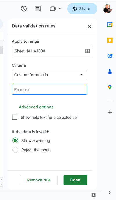
We will enter a custom formula in the Custom formula is field to restrict users from entering special characters.
Use REGEXMATCH in Data Validation to Restrict Special Characters
Enter the following custom formula in the Custom formula is field.
=REGEXMATCH(A1&"", "^[a-zA-Z0-9]*$")Then click Advanced options, select Reject the input, and click Done.
Please note one thing. Although we want to apply the rule to the entire range A1:A, the formula only needs to refer to the topmost cell in that range, which is A1.
The above formula allows only alphanumeric characters, thereby preventing users from entering special characters anywhere in the range A1:A.
In other words, it allows only uppercase letters, lowercase letters, and numbers.
Does the Above Rule Allow Spaces?
No. To allow spaces as well, use the following formula.
=REGEXMATCH(A1&"", "^[a-zA-Z0-9\s]*$")How Do I Restrict Only Specific Special Characters?
If you want to prevent users from entering only certain special characters, use the following formula.
=NOT(REGEXMATCH(A1&"", "[\&\$\%\#\@\!]"))This formula blocks only the characters listed inside the square brackets: &, $, %, #, @, and !.
FAQ
Can I Limit the Number of Characters in a Cell?
Yes. Restricting special characters is different from limiting the number of characters a user can enter.
To allow only alphanumeric characters and limit the entry to 10 characters, use the following custom formula in Data validation.
=REGEXMATCH(A1&"", "^[a-zA-Z0-9]{0,10}$")To limit the entry to 50 characters regardless of the characters used, use:
=LEN(A1)<=50How Do I Block Specific Special Characters and Limit the Number of Characters?
You can combine both conditions using the AND function.
For example, to block only &, $, %, #, @, and ! while limiting the input to 10 characters, use:
=AND(NOT(REGEXMATCH(A1&"", "[\&\$\%\#\@\!]")), LEN(A1)<=10)Note: A single Google Sheets cell can contain up to 50,000 characters.
