Quick Answer:
To highlight cells containing special characters in Google Sheets, use this custom formula in conditional formatting:

=LEN(TRIM(REGEXREPLACE(A1, "[A-Za-z0-9]", "")))>0

With the help of a custom rule, you can easily highlight any cell, column, or row that contains special characters in Google Sheets.

In this tutorial, special characters refer to anything other than letters (A–Z), numbers (0–9), and spaces. However, you can customize the formula to allow specific characters when needed.

Examples of Special Characters

Some common special characters include:

; < = > [ \ ] ^ _ ` { | } ~ ? @ ! & " # $ % ' ( ) * + , - . :

Foreign characters are also treated as special characters. For example, in the name “Anne Brontë”, the character ë will be detected.

Highlighting Cells that Contain Special Characters

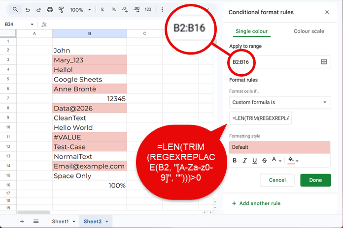
Assume you want to highlight cells with special characters in the range B2:B16.

Use the following formula in conditional formatting:

=LEN(TRIM(REGEXREPLACE(B2, "[A-Za-z0-9]", "")))>0

Steps:

1. Select your data range (e.g., B2:B16).
2. Go to Format > Conditional formatting.
3. Under Format cells if…, choose Custom formula is.
4. Enter the formula.
5. Choose a formatting style and click Done.

Highlight Entire Rows or Columns with Special Characters

Highlight Entire Columns

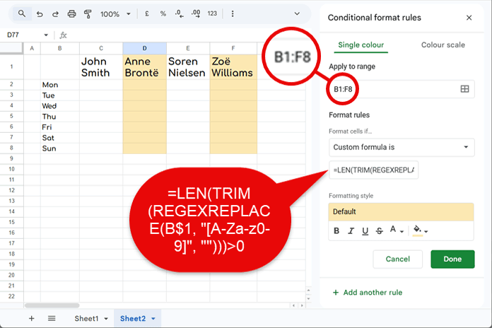
Assume your table is in the range B1:F8.

=LEN(TRIM(REGEXREPLACE(B$1, "[A-Za-z0-9]", "")))>0

• Detects special characters in row 1
• Highlights entire corresponding columns

Make sure the Apply to range covers your full dataset (e.g., B1:F8).

This ensures the formatting is applied to entire columns based on matches in the reference row (B1:F1).

Highlight Entire Rows

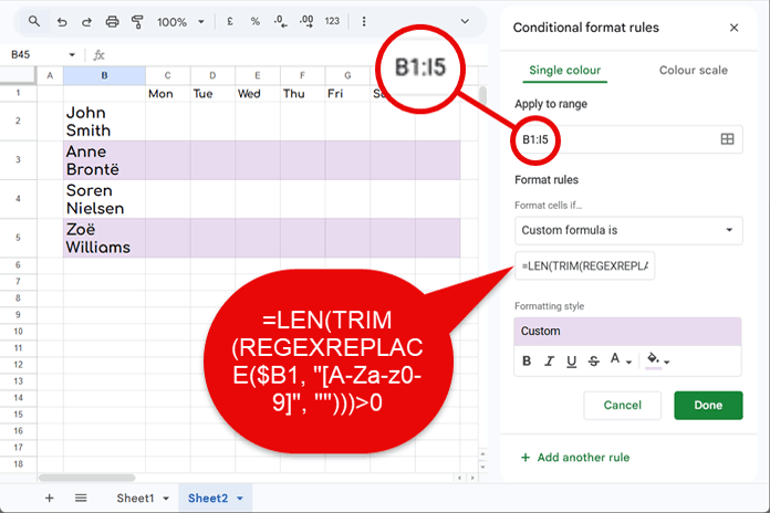
Assume your data range is B1:I5.

=LEN(TRIM(REGEXREPLACE($B1, "[A-Za-z0-9]", "")))>0

• Detects special characters in column B
• Highlights entire rows where matches occur

When highlighting entire rows, ensure the Apply to range covers your full dataset (e.g., B1:I5).
This allows the rule to apply across all columns, while the formula uses column B (via $B1) as the reference to determine which rows to highlight.

How This Formula Works

• REGEXREPLACE removes all alphanumeric characters
• TRIM removes extra spaces
• LEN counts the remaining characters

If the result is greater than 0, it indicates that the cell contains special characters, and the cell will be highlighted.

Exclude Specific Special Characters

To allow certain characters like _ or @, modify the formula:

=LEN(TRIM(REGEXREPLACE(A1, "[A-Za-z0-9@_]", "")))>0

You can add any characters inside the square brackets to exclude them from detection.

Conclusion

This tutorial is part of The Ultimate Guide to Conditional Formatting in Google Sheets, where you can explore 80+ practical formatting techniques, including advanced highlighting rules, real-world use cases, and optimization tips.

If you’re working extensively with data validation or cleanup, mastering these formulas can significantly improve your workflow.

Related Tutorials

• Restrict Entering Special Characters in Google Sheets (Data Validation)
• Insert Special Characters Without Add-on in Google Sheets
• Inserting Bullet Points in Google Sheets