The ISEVEN function in Google Sheets is categorized under the math function. Use this function to check the presence of even integer values in cells. It returns TRUE or FALSE based on the test value.

ISEVEN is effective in data analysis and can be part of combination formulas. In this Google Spreadsheet tutorial, I am explaining this simple function.

Syntax:

ISEVEN(value)

Here the argument value can be date or number. When you use a date, the date value will be taken into account.

Examples of the Use of ISEVEN Function in Google Sheets

The below ISEVEN formula will return TRUE since the number is even.

=ISEVEN(12)

Needless to say, an odd number as the value will result FALSE. What about the use of a date in the ISEVEN function in Google Sheets?

My system date today is 26/09/2018. See the below ISEVEN formula.

=ISEVEN(TODAY())

This formula returns FALSE simply because of the date value of the provided test date, which is an odd number.

=DATEVALUE(TODAY())

Result: 43369

You May Like: Learn All Popular Date Functions in Google Sheets.

How to Use ISEVEN Function in an Array

No doubt, you can use the ISEVEN with a range of values. The below example shows the same.

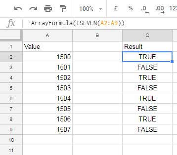
The ISEVEN function itself is not an array formula. So it’s a must to use the function ArrayFormula with it. But there is an exception to this rule.

If you use the function ISEVEN with any array functions, then the above rule is not relevant. The ISEVEN together with Filter is the best example of this.

How to get even numbers as output instead of TRUE or FALSE? See the answer under the title below.

The Use of ISEVEN in Filtering

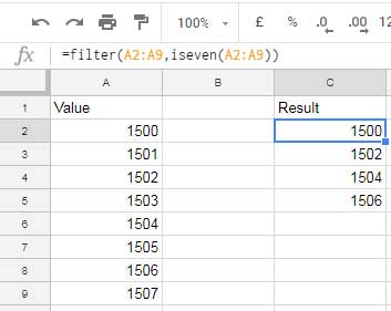
In the following example, the Filter formula filters only the even numbers in the given range.

ISEVEN in Conditional Formatting

It’s one of the functions that is famously being used in conditional formatting. You can use an ISEVEN formula to get alternating colors in the selected rows.

You May Also Like: How to Conditional Format Duplicates Across Sheet Tabs in Google Sheets.

Note: Actually, you can easily apply the same setting without formula from Format > Alternating colors.

Example:

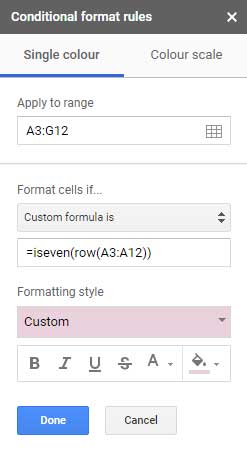
I want to apply alternating color in the range A3: A12. How to do that?

Select the range A3: A12 and go to the menu Format > Conditional formatting and apply the below formula rule.

Tip: The Zero is an even number!

How to Use Iseven with IF Logical Statement

You can test a value whether it’s even with IF and perform do this or do that based on it.

=if(iseven(A1),"even","odd")

In this, you can replace the test strings “even” or “odd” with other calculations. The calculation will be done based on the value in A1.

Must Read: Combined Use of IF, AND, OR Logical Functions.

Practical Use of the ISEVEN Function in Google Sheets

The below example shows how useful is the ISEVEN function in Google Sheets in certain data manipulation techniques.

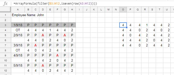
Here is part of an attendance sheet, which is not formatted correctly.

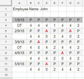
This data shows the present/absent status of an employee and his overtime hours. In this, how to filter all the number which is overtime hours?

You can see that cell C6, C10, and C12 which are missing the text “OT” even though that rows contain the overtime hours.

This data is not formatted well so it’s tough to apply a filter using the criterion “OT”. But you can use the filter formula as below.

Formula:

=ArrayFormula(filter(B3:H12,iseven(row(A3:H12))))

Result:

That’s all about how to use the ISEVEN function in Google Sheets.