A checked checkbox holds the value TRUE, while an unchecked checkbox holds the value FALSE in Google Sheets. You can use these TRUE/FALSE boolean values to check or uncheck a tick box based on another cell’s value dynamically. This tutorial will guide you through the steps to check/uncheck a tick box based on another cell.
How to Check or Uncheck a Tick Box Based on Another Cell in Google Sheets
If you want a tick box in cell A2 to be checked based on the value in cell B2, such as “Paid,” you can use this approach:
- Enter the formula
=B2="Paid"in cellA2. - While keeping
A2selected, go to Insert > Tick Box.
This setup ensures that the tick box in A2 gets checked when the value in B2 is “Paid” and unchecked when B2 contains any other value.
Auto-Toggling Multiple Tick Boxes
Can I Apply This to a Range of Tick Boxes?
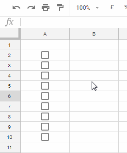
Yes! You can dynamically check or uncheck multiple tick boxes based on the values in another column. For example, to toggle the tick boxes in A2:A10 based on the values in B2:B10, follow these steps:
- Clear any existing data in the range
A2:A10. - Enter the following formula in cell
A2:=ArrayFormula(B2:B10="Paid") - Select the range
A2:A10. - Go to Insert > Tick Box.
This will create a range of tick boxes that automatically toggle based on whether the corresponding cells in B2:B10 contain the value “Paid.”
Real-Life Examples: Check or Uncheck Tick Boxes Based on Cell Values
Example 1: Toggle Tick Boxes for Payments
Imagine you have a column for payment amounts. You want the tick boxes in A2:A10 to be checked when a payment is received (i.e., the amount in B2:B10 is greater than 0). Use this formula in A2:
=ArrayFormula(B2:B10>0)Then select A2:A10 and go to Insert > Tick Box.
Example 2: Lookup and Toggle Tick Boxes
You can use lookup functions in Google Sheets to toggle tick boxes dynamically. For instance, if you have a list of items in column A and a table in the range D2:E8 that categorizes items (e.g., “Fruits” and “Vegetables”), you can insert tick boxes based on categories.
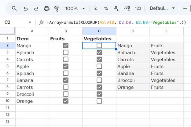
To insert checked tick boxes for all items in A2:A10 that are categorized as “Fruits”:
- Enter the following formula in cell
B2:=ArrayFormula(XLOOKUP(A2:A10, D2:D8, E2:E8="Fruits")) - Select
B2:B10. - Go to Insert > Tick Box.
Where in the formula:
A2:A10is the search_key range.D2:D8is the lookup range.E2:E8="Fruits"is the result range, which containsTRUEfor “Fruits” andFALSEfor other items.
For vegetables, modify the formula:
=ArrayFormula(XLOOKUP(A2:A10, D2:D8, E2:E8="Vegetables"))You can create separate tick box columns for each category if needed. In that case, insert the above formula in cell C2 instead of modifying the formula in cell B2.
Additional Resources
- Assign Values to Tick Boxes and Calculate the Total in Google Sheets
- Change the Tick Box Color While Toggling in Google Sheets
- 10 Best Tick Box Tips and Tricks in Google Sheets
- Highlighting Multiple Groups and Control Tick Boxes in Google Sheets
- Create a List from Multiple Column Checked Tick Boxes in Google Sheets


I need a checkbox to auto-check when any cells in a range contain the word “Get”.
Is this doable?
I need the C32 checkbox to check if any cell in A3:A14 contains the word “get” in them.
Hi, Missy Jennings,
I’ve keyed in the following solution in cell C32. Please check your Sheet.
=IFNA(XMATCH("*get*",A3:A14,2))>=1Hi,
This may not be able to be done, but I am hopeful it is.
I want to create a competency form for my trainers to fill out every time a trainee completes a competency, and it will then import the data from the form to a sheet inside the workbook.
From there, I want a check box that will search through the names of the form responses and tick a checkbox on an overview sheet corresponding with the name, and the competency completed.
I would like them to automatically update the checkboxes, whether every time a response is submitted or whenever I don’t mind.
I hope this makes sense. I can try to attach photos of each sheet to make it a little easier to understand if this doesn’t make sense.
Hi, Tom,
Can you share a copy/sample of your sheet instead of screenshots?
I’ll try then.
This is all really helpful.
Essentially, I want to ensure that only one of the three tick boxes is able to be ticked at a given time.
I’m still trying to figure out my footing when it comes to formulas, so grace is appreciated!
Hi, Lizzy,
It doesn’t seem possible since the formula applied cell becomes unclickable.
The workaround is to limit entering values in those cells, e.g., if C2, D2, and E2 are the cells, you can use the following formula in Data Validation > Criteria > Custom Formula field.
=COUNTA($C$2:$E$2)<2Check "Reject input," and the cell range must be C2:E2.
It will make users enter a value (e.g., a ✔ symbol) in only one of the cells in C2:E2.
I have a checkbox in column Z. I have a date (birthdate) in the H column.
How can I have the checkbox check automatically when the age of the person is below the age of 16?
I can add a column that calculates the date (we’ll say column AA).
Hi, DeeMarie,
I assume the data is as follows.
DOB in H2:H
Tick boxes in Z2:Z.
Then in Z2, insert the following Datediff formula and copy it down.
=datedif(H2,today(),"Y")<16Thank you for this.
I’m wondering though, is it possible to have a checkbox be ticked if one or more checkboxes on other sheets get ticked?
For example, if I have three people out of six with their own sheets that check a box, can a box on another sheet get ticked?
Hi, Ela,
Are you referring to six workbooks (Sheets) or that many tabs within a single workbook?
In both cases, we might be able to do that. Please elaborate and feel free to share a sample of your Sheet below.
It’s one workbook with several tabs inside it.
Hi, Ela,
Yep! It seems possible.
Example:
Master Sheet:
Sheet1 is the master sheet that contains the following data.
A2:A – the candidates’ names
B1, C1, and D1 – tab names Joe, Jan, and Sharon (interviewers).
Other Sheets:
Joe (tab name)
Jan (tab name)
Sharon (tab name)
These three sheets contain the following data.
A1:A – the candidates’ names
F1:F – tick boxes (interview result column)
In Sheet1!B2, i.e., master sheet, insert the following formula and copy it to C2 and D2.
=ArrayFormula(ifna(vlookup($A$2:$A,indirect("'"&B1&"'!A1:F"),6,0)))Select B2:D and apply Insert >Tick box.
Thank you for these tutorials.
So is it true that it is not possible to make an “Uncheck All” box (or drop-down selection) while allowing the other boxes to be interactive?
Hi, Josh,
For that, you can get the help of Macros.
Steps:
1. Go to Extensions > Macros > Record Macro.
2. On the dialog box that appears, check/enable “Use absolute references.”
3. Select the tick boxes on the sheet.
4. Tap the Space bar twice.
5. Save the Macro.
Thank you, Prashanth! I’ve very appreciative of the wealth of knowledge you have here.
I’m having an issue with the formula when I replace the word “Paid” with a value in another cell (i.e., “24”). Is there a way to correct this?
Hi, Tyler,
I am not clear about your question. Can you elaborate or share an editable sheet via “Reply” below.
Hi,
How can I make the tick boxes in column A to be checked automatically if the adjacent cell from row B is checked?
For example: If I check B5, then A5 to be checked automatically as well.
Thank you.
Hi, Alex,
Insert tick box in cells A5 and B5. Then in A5 type the following formula and hit enter.
=B5=TRUEThat’s it!
When you check B5, A5 will be checked automatically. But the problem is A5 won’t be interactive anymore!
I must be missing something. If I type a formula into a cell with a checkbox then the checkbox goes away. How do you get it to stay as a checkbox?
How could you code this into a script so that when cell C contains the text “Approved” the checkbox in cell D is checked? I enjoy reading your clear descriptions and find them very useful!
Hi, SmilinJack,
Empty D1:D. Then insert the below formula (array formula) in D1.
=ArrayFormula(if(len(C1:C),if(C1:C="checked",TRUE,FALSE),))Select the values in D1:D, click on Insert > Tick box.
Is it possible to automatically check a tick box if all other tick boxes in a specific range are checked? For example, I want the tick box at A4 to be checked if the tick boxes from A5 to A11 are all checked.
Hi, iowaniklas,
Yes, it’s possible using the below formula in cell A4.
=if(COUNTIF(A5:A11,TRUE)=7,TRUE,FALSE)Thanks for this Prashanth – this was super helpful! However, I need to go one step further with my formula if possible…
Using your example of:
=if(B2="Paid",1,0)I’ve modified this to take in to account a couple of other factors in my data set. Namely:
– Another worksheet in the same workbook happens to be a ‘form responses’ sheet.
– Full column instead of just one other cell.
– Boolean search modifier * to return a root word/stem/truncation value.
This is the formula I’ve entered in:
=if('OTHERSHEET'!B:B="*DSC*",1,0)When I enter this, it seems to break the formula so it doesn’t work. Although there is no error message, it always generates a FALSE or 0 value in the checkbox cell even when the criteria should read as TRUE / 0 based on the targetted cell.
Do you have any advice on whether this is possible and if so, how I can modify my formula?
Thank you!
H
Hi, Helena M,
As far as I know, it’s not possible. Your formula is not correctly coded. Even if it’s correct, the formula would return #REF! error as it won’t overwrite the tickboxes.
Please note the below two points that would help you advance in Google Sheets.
To use a full column instead of just one other cell, you must enter your formula as an Array Formula. Either wrap your IF formula with the ARRAYFORMULA() function or hit Ctrl+Shift+Enter.
To return a root word/stem/truncation value in IF, do not use the
*wildcard character. The said function doesn’t support it. Then?Please follow this – Partial Match in IF Function in Google Sheets As Wildcard Alternative.
Is it possible if the tick box is ticked manually or automatically by referencing other calls at the same time?
Hi, Azahari,
It’s not possible as there is a formula in the tick box cell. So you can’t manually check it.
Best,
Thank you for this, but I do have some question for the
=if(B2="Paid", TRUE, FALSE)formulaWhat if I have a drop-down option with “venmo”, “cash”, “paypall”, “other” and want the box to be checked if any option is selected remains unchecked if no value is selected?
I’m having issues “grouping cells” on Google Sheets, and Excel is not really an option for me.
Please help!
Hi, JD,
You can use this formula that uses OR in IF.
=if(or(B2="venmo",B2="cash",B2="paypall",B2="other"),TRUE,FALSE)Best,
Thanks so much for the IF statement modification of the checkbox! It was exactly what I needed to make a list beautiful and matching some other checkboxes.