You are not permitted to use wildcard characters to find a partial match in the IF function in Google Sheets. However, it’s still achievable through a different approach. Of course, I can provide you with examples of this. Additionally, there are some more important additional tips covered in this tutorial.

Here, you can learn how to use the IF function to find a partial match in Google Sheets, such as:

• IF in a partial match.
• Use of IF and AND in a partial match.
• Lastly, the utilization of IF and OR in a partial match.

How to Do a Partial Match in IF Function in Google Sheets

Here is a standard IF formula that checks the value in cell A1 and returns a tick mark if the value matches the IF condition.

The value in cell A1 for this test is “Gr. 0001.55” (note the space after “Gr.”). Either of the following formulas would return a check mark (✔).

=IF(A1="Gr. 0001.55", CHAR(10004),)
=IF(A1="Gr. 0001.55", "✔",)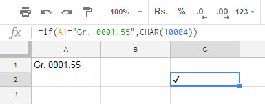

Now, I want a partial match of the value in cell A1. In other words, I need an IF formula in cell C2 that evaluates/tests whether cell A1 contains “Gr. 0001”, and returns a tick mark if it does.

Formula 1:

=IF(A1="Gr. 0001", CHAR(10004),)

This formula will return blank since the value in cell A1 is “Gr. 0001.55”. If you think you can use wildcard characters to do a partial match in the IF function in Google Sheets, you are mistaken!

Here is the solution. You can use either of the following formulas (Formula 2 or Formula 3), which utilize the FIND function for a partial match.

Syntax of the FIND function: FIND(search_for, text_to_search, [starting_at])

Formula 2 (Partial Match in IF):

=IF(IFERROR(FIND("Gr. 0001", A1))>=1, CHAR(10004),)

Formula 3 (Partial Match in IF):

=IF(COUNT(FIND("Gr. 0001", A1))>=1, CHAR(10004),)

The FIND formula returns:

• 1, if the search_for (the keyword “Gr. 0001”) is at the beginning of the text_to_search (“Gr. 0001.55”).
• Greater than 1 if the search_for is not at the beginning.
• If the search_for is not present (no partial match), then the formula would return a VALUE! error.

In the first formula, the FIND returns either a number (partial match) or an error (no partial match). The IFERROR removes the error. The IF evaluates this result.

But in the second formula, I’ve adopted a different approach. There, I’ve used the COUNT function. The COUNT returns 1 if the output of the FIND is greater than or equal to 1, else it would return 0. The IF evaluates this output.

Note: The FIND function matches the text in case-sensitive mode. If you want a case-insensitive match, use the SEARCH function instead.

How to Do Partial Match in IF and OR Logical Functions in Google Sheets

We can use the OR logical function in Google Sheets to return a value if any of the conditions are TRUE. First, let’s look at a normal OR logical test:

=IF(OR(A1="Gr. 0001.55", B1="Gr. 0001.55", C1="Gr. 0001.55"), CHAR(10004),)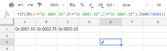

This formula returns a tick mark if any of the values in cells A1, B1, or C1 match “Gr. 0001.55”.

However, it may not work for a partial match. You can use the below formula to perform a partial match in IF and OR functions in Google Sheets.

Formula 4:

=ArrayFormula(IF(COUNT(FIND("Gr. 0001", A1:C1))>=1, CHAR(10004),))

This formula aligns with our partial match formula used in the earlier example (formula 3). Therefore, I won’t delve into the details again. The difference here lies in the multiple cells/range in FIND. Thus, I’ve used the ArrayFormula here.

How to Do Partial Match in IF and AND Logical Functions in Google Sheets

Use the logical function AND to return a value (tick mark) when all the conditions are TRUE. In our example, if the values in cells A1, B1, and C1 have a partial match, we want the formula to return a tick mark. Below is the formula:

Formula 5:

=ArrayFormula(IF(COUNT(FIND("Gr. 0001", A1:C1))=COLUMNS(A1:C1), CHAR(10004),))

In this formula, there is only one difference from the OR partial match formula. What is that?

Here, instead of using “>=1”, I’ve employed the COLUMNS formula. Actually, you can substitute the number 3 there instead of utilizing the COLUMNS formula, as the COLUMNS formula itself returns the number 3.

That concludes the discussion on Partial Match in the IF Function in Google Sheets.

Since wildcard characters are not effective for partial matching in IF logical tests, we can explore the above alternatives. Enjoy!

Resources

1. Formula to Find Partial Match in Two Columns in Google Sheets
2. Partial Match in Vlookup in Google Sheets [Text, Numeric, and Date]
3. CONTAINS Substring Match in Google Sheets Query for Partial Match
4. Highlight Partial Matching Duplicates in Google Sheets
5. Lookup Last Partial Occurrence in a List in Google Sheets
6. Filter Out Matching Keywords in Google Sheets – Partial or Full Match
7. How to Custom Sort By Partial Match in Google Sheets