The VLOOKUP function accepts wildcard characters in the search key. Therefore, achieving a partial match in VLOOKUP is straightforward in Google Sheets.
Some of you may already be familiar with using wildcards in Google Sheets functions. However, the importance of the partial match in VLOOKUP lies in your specific requirements:
- Whether you want to use the search key in a cell reference or hardcode it in the formula.
- Whether you require a case-sensitive partial match, where the wildcard won’t be utilized.
We will address both in this walkthrough guide with simple steps.
Partial Match in VLOOKUP Using Wildcard Characters
Let’s assume you have a small team of employees, each with a unique first name.
Your data contains employee names in column A (full names), their designations in column B, and attendance in the current month in column C.
| Full Name | Designation | Attendance |
| John Smith | Accountant | 22 |
| Alice Johnson | Engineer | 18 |
| Michael Brown | Teacher | 18 |
| Emily Davis | Nurse | 22 |
| David Taylor | Lawyer | 18 |
How do you look up their first names in column A and retrieve their attendance from column C?
This is where the relevance of partial match in VLOOKUP is apparent.
Syntax of the VLOOKUP Function in Google Sheets:
VLOOKUP(search_key, range, index, [is_sorted])Example
The following VLOOKUP formula will partially match “Alice” in the range A2:C6 and return the value (attendance) from the third column.
=VLOOKUP("*Alice*", A2:C6, 3, FALSE) // returns 18Remember, VLOOKUP searches the key in the first column of the range.
Alternatively, you can enter *Alice* in any cell, for example, cell E2, and use the formula as follows:
=VLOOKUP(E2, A2:C6, 3, FALSE)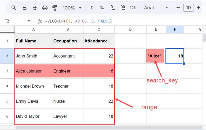
Notes:
- To search for names starting with “Alice”, you can use
"Alice*". - To search for names ending with “Johnson”, you can use
"*Johnson". - To search for a word that appears anywhere in the text, you can use
"*text*". Replace “text” with the word you want to search for.
The above notes are applicable when you enter the search_key within the formula. When you prefer cell reference, enter the search_key in a cell without double quotes.
Case-Sensitive Partial Match in VLOOKUP
VLOOKUP is typically a case-insensitive function in Google Sheets, meaning that capital and small case letters don’t make any difference in the search.
However, case sensitivity in a partial match becomes crucial in VLOOKUP when the range contains text entries with different cases (uppercase and lowercase), such as product codes or identifiers.
How do you perform a case-sensitive partial match in VLOOKUP?
You can achieve this by virtually modifying the range using a combination of HSTACK and REGEXMATCH.
In the following example, let’s say we need to partially search the key “XYz” in the range A2:B5 and return the result from the second column. This requires a case-sensitive VLOOKUP.
Step-by-Step Instructions
=ArrayFormula(REGEXMATCH(A2:A5, "XYz"))– This REGEXMATCH formula partially matches the key “XYz” and returns TRUE for matches and FALSE for mismatches.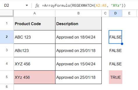
- Use HSTACK to combine this range with the rest of the range in the table, which is B2:B5.
=HSTACK(ArrayFormula(REGEXMATCH(A2:A5, "XYz")), B2:B5)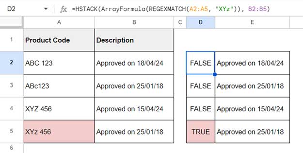
- In this table, search for TRUE using VLOOKUP.
=VLOOKUP(
   TRUE,
   HSTACK(ArrayFormula(REGEXMATCH(A2:A5, "XYz")), B2:B5),
   2,
   FALSE
)
This represents a case-sensitive partial match in VLOOKUP.
Notes:
REGEXMATCH(A2:A5, "XYz")– searches anywhere in the text.REGEXMATCH(A2:A5, "^XYz")– matches strings starting with “XYZ”.REGEXMATCH(A2:A5, "XYz$") – matches strings ending with “XYZ”.
Resources
Here are some related tutorials regarding partial matches in Google Sheets.


