Here is a workaround to use wildcards in Vlookup Range in Google Sheets. The workaround shows the alternative to asterisk wildcard use in the range.

The WILDCARDS are for partial matching in spreadsheet formulas. But it won’t work with all the functions.

Regarding Vlookup, as far as I know from my extensive testing, we can only ‘directly’ use WILDCARDS with the search key.

The search key is the first argument in Google Sheets Vlookup. The second argument is the range.

From the below syntax, you can understand the positioning of the ‘arguments’ in the function.

Syntax: VLOOKUP(search_key, range, index, [is_sorted])

As a side note, I’ve already explained the use of wildcards with the search_key in Vlookup in Google Sheets. Here is that post – Partial Match in Vlookup in Google Sheets [Text, Numeric and Date].

We can’t use the wildcards in the Vlookup range in Google Sheets. To overcome this, we should use some kinds of workaround formula.

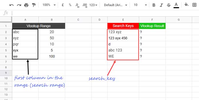
For example, if we want to use the search_key “123 xyz” to search it in the range A2:A and return the value from B2:B, we will possibly use the below Vlookup in F2.

=vlookup(E2,A2:B,2,0)

No doubt, it would return an #N/A error indicating the search key is not present in the range.

We can’t use wildcards in the Vlookup range as below in Google Sheets!

=ArrayFormula(vlookup(E2,{"*"&A2:A&"*",B2:B},2,0))

You will get the same above error.

How to Use Wildcards in Vlookup Range in Google Sheets

Using three functions as a combination we can solve this issue. The functions don’t involve Vlookup. The said functions are Regexmatch, Filter, and Index.

Must Check: Google Sheets Function Guide [Quickly Learn All Popular Functions].

Use the below formula, as an alternative to the wildcards in Vlookup range in Google Sheets, in cell F2, and drag down.

=index(
     FILTER(
        $B$2:$B,
        REGEXMATCH(lower(E2),lower($A$2:$A))
     ),
     1,1
)

It is also called partial RANGE match in Vlookup in Google Sheets. Let’s learn the formula in detail below.

The role of the LOWER function is minimal in the formula as it’s for making the formula case insensitive.

Below, I am explaining the functionality of the other Google Sheets functions present in detail.

We must read the formula from the middle, and that is the Regexmatch formula here.

Regexmatch to Partial Match in Vlookup Range in Google Sheets

Formula Part 1:

REGEXMATCH(lower(E2),lower($A$2:$A))

Don’t try this formula in your sheet as it won’t return the correct result.

Using the above part, what we want is to partially match the value in the cell E2 (“123 xyz”) in the range A2:A.

Please note that the above part of the formula is within the FILTER in the main formula. Outside FILTER, to test the above Regexmatch formula, you must use it as an array formula as below.

=ArrayFormula(REGEXMATCH(lower(E2),lower($A$2:$A)))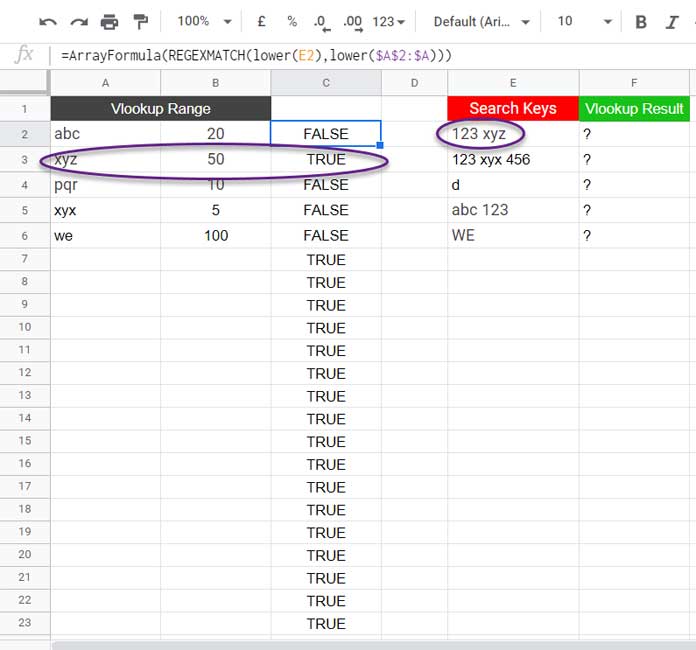

The formula returns TRUE in the row that contains the partial match of the search key, i.e., “123 xyz”, in the Vlookup range (we can ignore the TRUE in blank rows).

FILTER Only the Boolean TRUE Values

It is the main part of the ‘workaround’ use of wildcards in the Vlookup search range in Google Sheets.

Let’s filter B2:B, the Vlookup result (index) column, wherever Regexmatch returns the Boolean TRUE values. The below formula does that.

Formula Part 1 and 2:

=filter($B$2:$B,ArrayFormula(REGEXMATCH(lower(E2),lower($A$2:$A))))

As per the FILTER syntax, the above Regexmatch formula is the ‘condition’ here.

Syntax: FILTER(range, condition1)

Note:- If you want to filter FALSE values, then you should specify that in the condition. For TRUE, it’s not necessary.

We can remove the ArrayFormula as the Regexmatch is within Filter. So here is the shortened form of the above part 1 and 2 formula.

=filter($B$2:$B,REGEXMATCH(lower(E2),lower($A$2:$A)))

What’s the Role of the Index Then in the Final Formula?

Sometimes, the above Filter may return two or more values in case there are multiple matches of the same search_key.

We Want the first one as per the Vlookup standard.

The INDEX does that part wonderfully.

That’s all about the use of Wildcards in Vlookup Search Range in Google Sheets.

Thanks for the stay. Enjoy!