How can we enforce that a user must enter values from a list in the same order as the list in Google Sheets?
With Data Validation in Google Sheets, we can control how data is entered in a cell or range. By using a data validation drop-down from a range, we can ensure entries follow the order of the original list while still allowing repeats.
In other words, you can make sure a user only enters data from a given list — and that each entry follows these rules:
- The entered values appear in the same order as the list.
- Values may repeat.
In this Google Sheets tutorial, you’ll learn step-by-step how to enter values from a list in order using a simple but effective trick.
Example: Enforce Entry Order from a List in Google Sheets
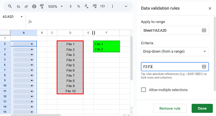
Here’s an example list (in D2:D11) containing file names from File 1 to File 10:
File 1
File 2
File 3
File 4
File 5
File 6
File 7
File 8
File 9
File 10
The list can contain any values — file names are just an example. It could be product names, book titles, item codes, station names, flight numbers, or any ordered list.
Our goal is to restrict entries in column A so that:
- Values must come from the list in
D2:D11. - The order of entries in column
Amatches the list order. - Values can repeat.
For instance, if File 3 has already been entered, the next valid entry must be either File 3 (repeat) or File 4 (next in sequence). If File 4 appears before File 3, it’s invalid.
The Logic Behind the Method
We’ll use a data validation drop-down that updates dynamically so that each row only offers two valid options:
- The same value as the row above (for repeats).
- The next value in the source list.
To achieve this, we’ll use two helper cells containing formulas that return the “current” value and the “next” value. The drop-down will reference these helpers instead of the full list.
Step 1: Formula 1 — Last Value from Column A or First Value from the List
Enter this formula in cell F2:
=IFERROR(CHOOSEROWS(TOCOL(UNIQUE(A2:A), 3), -1), D2)Explanation:
UNIQUE(A2:A)– Removes duplicates from column A.TOCOL(..., 3)– Flattens the list and removes blank cells.CHOOSEROWS(..., -1)– Returns the last value from the cleaned list.
If column A is empty, it will return the first value from your source list.
Step 2: Formula 2 — Next Value in the List
In cell F3, enter:
=OFFSET(XLOOKUP(F2, D2:D11, D2:D11), 1, 0)Explanation:
XLOOKUP(F2, D2:D11, D2:D11)– Finds the current value (F2) in the list.OFFSET(..., 1, 0)– Returns the value one row below (the “next” value).
Step 3: Create the Drop-Down List
- Select the range where you want to enforce the rule (e.g.,
A2:A20). - Go to Insert > Drop-down.
- Under Criteria, choose Drop-down (from a range).
- Enter the range
F2:F3(the two helper cells). - Click Done.
Now, any user entering data in column A can only select the same value as above or the next value in the original list, ensuring the correct sequence.
Sample Sheet
Related Resources
- Distinct Values in Drop-Down List in Google Sheets
- Google Sheets: Add an ‘All’ Option to a Drop-down from Range
- Create a Drop-Down Menu From Multiple Ranges in Google Sheets
- Highlight Invalid Entries in Drop-down Lists in Google Sheets
- How to Use Relative Reference in Drop-Down List in Google Sheets


Remark 2:
Let’s say, you click the dropdown button in cell A2 and you choose the value “File 1”. Next, you click the dropdown button in cell A3 and you choose the value “File 2”.
At this moment, you realize you made a mistake: cell A3 should have been “File 1” again. Now, when you click the dropdown button in cell A3 again, you now have only the values “File 2” and “File 3”.
Manually correcting using “backspace” to the value “File 1” will not be accepted (as expected). The only way to get “File 1” into cell A3, is to delete the contents of cell A3 and choose “File 1” again from the dropdown button (or type it)… That works but is a bit annoying…
Hi, Jurgen Lamsens,
That’s because the formulas in cells F2 and F3 uses the drop-down values in the calculation.
If you want, you can alert the user about the same by putting a validation help text like “wrong selection? delete the value and try again”.
Hi P,
I was that reader… 😉
1. Thanks again for this nice solution. When only “File 1” is entered in “A2”, there is no problem as “File 1” is in the range of “F2:3” at that moment. Entering “File 2” on “A3” however, makes “File 1” not fit in the dynamic range “F2:3” anymore. Consequence: those red “Invalid” messages. Any idea how to avoid them?
2. I found an alternative solution in Excel, but it does not work when ported to Google Sheets. I’ll send you an e-mail. Would you be so kind to look at that solution and try to find why it does not work in a Google Sheet? Should you find it: please feel free to maybe use it in an article: it is based on “dependent drop-down lists”.
Hi, Jurgen Lamsens,
I don’t find a way to remove those invalid messages 🙁
The only way is to export the values to another sheet in that file like;
={Sheet1!A2:A20}or
=ArrayFormula(Sheet1!A2:A20)which you may already know.