To remove or replace the last character from a string in Google Sheets, you can utilize either a formula or the Find and Replace command.
When using a formula, several options are available, including the REGEXREPLACE function, or combinations such as LEN + REPLACE, LEN + LEFT, or LEN + MID.
It’s essential to note that the formula doesn’t modify the original text; instead, it executes the operation and displays the result in another cell or cell range.
One advantage of using the menu command is its ability to modify the existing data directly. We will employ a regular expression within the Find dialog box to identify the last character and replace it with either null or a character of your choice.
Removing or Replacing the Last Character Using Find and Replace in Google Sheets
In the following example, we have fruit names like “apples,” “mangos,” “bananas,” and “grapes” in cells C2 to C5.
Let’s explore how to remove the last characters from these fruit names using the Find and Replace dialog box in Google Sheets. Follow these step-by-step instructions:
- Select cells C2 to C5.
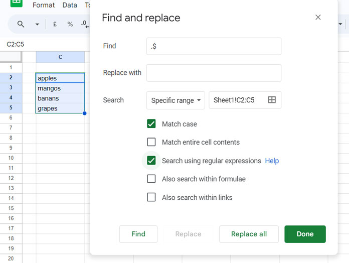
- Click on Edit > Find and Replace to open the dialog box. Alternatively, you can use the Google Sheets keyboard shortcuts
Ctrl + hin Windows orCommand + Shift + hon Mac. - In the field next to “Find,” enter
.$ - Leave the field next to “Replace with” empty.
- Choose “Specific range” from the drop-down next to “Search.”
- Check both “Search using regular expressions” and “Match case” (note: “Match case” may be automatically selected when choosing “Search using regular expressions”).
- Click the “Replace all” button.
- Click “Done.”
This is the fastest method to remove the last character from a list of strings in Google Sheets.
If you wish to replace the last character with another character, enter that character or characters in the “Replace with” field.
Formula Options
As I mentioned at the beginning of this tutorial, there are several formula options available to remove the last character in a string.
Utilizing the REGEXREPLACE Function to Remove or Replace the Last Character
=REGEXREPLACE(C2, ".$", "")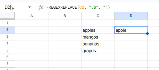
This follows the syntax REGEXREPLACE(text, regular_expression, replacement):
text: C2regular_expression:.$(.matches any character except for line terminators, and$asserts position at the end of a line)replacement: “”
This formula removes the last character from the string in cell C2.
If you want to replace the last character, specify the replacement in the argument. For example, using “_2” as the replacement will return “apple_2”.
To remove or replace the last characters in the range C2:C5, use the above REGEXREPLACE as an array formula:
=ArrayFormula(REGEXREPLACE(C2:C5, ".$", ""))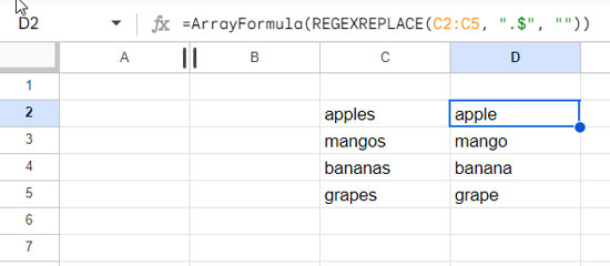
Utilizing LEN and REPLACE Functions Combo to Remove or Replace the Last Character
This is the second formula option to remove or replace the last character in a string or a list of strings.
The following combination will remove the last character in the string in cell C2:
=REPLACE(C2, LEN(C2), 1, "")The LEN function returns the number of characters in the string in cell C2, which corresponds to the position of the last character.
The REPLACE function then replaces the character in that position with a new text, specified here as "".
Syntax: REPLACE(text, position, length, new_text)
text: C2position: LEN(C2)length: 1 (one character)new_text: “”
If you want to replace the last character, specify the replacement in the argument. For example, using “_2” as the new_text will return “apple_2”.
To use it in an array, for instance in the range C2:C5, apply the following formula:
=ArrayFormula(REPLACE(C2:C5, LEN(C2:C5), 1, ""))Utilizing LEN and LEFT Functions Combo to Remove the Last Character
Here is the widely used combo to remove the last character from a string in Google Sheets as well as in Excel:
=LEFT(C2, LEN(C2)-1)The LEFT function returns LEN(C2)-1 characters from the left of the string.
Syntax: LEFT(string, [number_of_characters])
To apply this to a list, for example, C2:C5, use it as follows:
=ArrayFormula(LEFT(C2:C5, LEN(C2:C5)-1))Utilizing LEN and MID Functions Combo to Remove the Last Character
This combo is similar to LEN and LEFT.
=MID(C2, 1, LEN(C2)-1)Syntax: MID(string, starting_at, extract_length)
Here, the MID function returns LEN(C2)-1 characters starting at 1.
To apply this to a list, for example, C2:C5, use it as follows:
=ArrayFormula(MID(C2:C5, 1, LEN(C2:C5)-1))Resources
Here are some other tutorials covering similar topics, including character replacement and additional tips and tricks.
- Regex to Replace the Last Occurrence of a Character in Google Sheets
- How to Group a Column Based on First Few Characters in Google Sheets
- How to Remove the First N Characters in Google Sheets
- How to Check First N Characters Are Caps or Small in a List in Google Sheets
- Make Duplicates to Unique by Assigning Extra Characters in Google Sheets
- Insert Delimiter into a Text After N or Every N Character in Google Sheets
- Remove Repeated Characters from the End of Strings in Google Sheets


