IF and VLOOKUP are two standalone functions in Google Sheets. The IF function handles logical tests, enabling decision-making based on conditions, while VLOOKUP excels at retrieving data from vertical data ranges.
For example, IF can be used to determine whether the total sales from a region meet a set target. Suppose the total sales amount is in cell A1 and the target is 1000. The following formula will perform the test: =IF(A1>=1000, "Achieved", "Trailing"). This formula follows the syntax: IF(logical_expression, value_if_true, value_if_false).
The purpose of VLOOKUP is to retrieve a value from a table. For instance, if you want to find the salary drawn by an employee from a table containing employee names and salaries in columns A and B respectively, you can use =VLOOKUP("employee_name", A:B, 2, FALSE). This formula adheres to the syntax: VLOOKUP(search_key, range, index, [is_sorted]).
IF and VLOOKUP combination in Google Sheets offers a dynamic formula for customized data retrieval at your fingertips. By leveraging IF’s logical tests, we can control VLOOKUP’s behavior, tailoring results to specific criteria.
Join us as we dive in and discover how this dynamic duo can elevate your spreadsheet game!
IF and VLOOKUP Combination for Switching Lookup Tables in Google Sheets
Assume you have two tables: one containing data about fruits and the other about vegetables.
The range for Table #1 is A3:B7, and for Table #2, it’s D3:E6. In both tables, the first column holds the item names, and the second column contains their prices. You want to look up the price of a particular item using these tables.

Here’s how the IF and VLOOKUP combination works in this scenario:
Enter the table name (a meaningful name relevant to your data) you want to look up in cell H3. If you want to look up in the first table, enter “Fruits”; if you want to look up in the second table, enter “Vegetables”.
Specify the criterion in cell H4. For example, if you entered “Fruits” in H3 and “Avocado” in H4, use the following formula to dynamically return the price of “Avocado” from Table #1:
=VLOOKUP(H4, IF(H3="Fruits", A3:B7, D3:E6), 2, FALSE)When you want to find the price of “Spinach”, enter “Vegetables” in cell H3 and “Spinach” in cell H4. No changes are needed to the formula.
Alternative Solution:
Create two named ranges with the names “fruits” and “vegetables” as detailed here, and then use this formula:
=VLOOKUP(H4, INDIRECT(H3), 2, FALSE)Identifying Error Values in VLOOKUP Result Range
To rectify errors in the VLOOKUP result caused by the absence of the search key in the first column of the range, we can utilize the IFNA function. I advise against using the IFERROR function as it will conceal all error types.
Now, let’s delve into a less common scenario.
Suppose the search key exists in the lookup range, but the result column contains an error corresponding to the search key. In this case, VLOOKUP will yield an error.
If the result range displays an #N/A error, VLOOKUP will return that error. It might lead you to believe that the search key is absent. However, we can manage this situation using a combination of IF, MATCH, and VLOOKUP in Google Sheets.
Example of IF, MATCH, and VLOOKUP Combination in Google Sheets
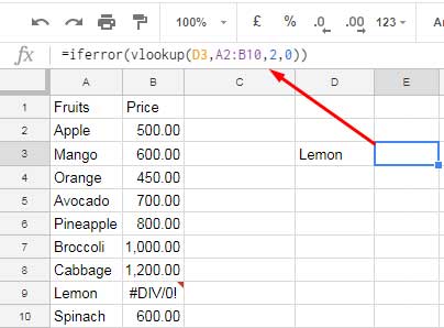
In the following scenario, the search key is “Lemon” in cell D3, which exists in the lookup range A2:B10.
The VLOOKUP formula provided, =VLOOKUP(D3, A2:B10, 2, 0), will generate a #DIV/O error since the result range contains an error corresponding to “Lemon”.
While you can make the result blank by applying IFERROR, I don’t recommend it.

Instead, here’s what we’ll do: First, we’ll match the search key using the MATCH function:
=MATCH(D3, A2:A10, FALSE)Then, we’ll incorporate that into an IF function:
=IF(
   MATCH(D3, A2:A10, FALSE),
   IFERROR(VLOOKUP(D3, A2:B10, 2, 0), "Result range has an issue"),
   ""
)
Here’s how this IF, MATCH, and VLOOKUP combination operates:
- If the search key is present, the IF executes the VLOOKUP. If the result is an error, the IFERROR returns “Result range has an issue”.
- If the search key is not present, the formula will return an #N/A error. If you want to avoid that error, wrap the MATCH function with IFNA like this:
IFNA(MATCH(D3, A2:A10, FALSE),)
Alternative Solution:
You can replace the errors in the range using IFERROR and utilize that modified range in VLOOKUP as follows:
=VLOOKUP(D3, IFERROR(A2:B10, "Issue in the range"), 2, FALSE)IF and VLOOKUP Combination for Evaluating Lookup Results with Comparison Operators
In Google Sheets, the comparison operators and equivalent functions are:
| Operator Name | Symbol | Function Name |
| Equal to | = | EQ |
| Not equal to | <> | NE |
| Greater than | > | GT |
| Less than | < | LT |
| Greater than or equal to | >= | GTE |
| Less than or equal to | <= | LTE |
These operators are commonly used in formulas to compare values and evaluate conditions. Here’s how to use them in an IF and VLOOKUP combination:
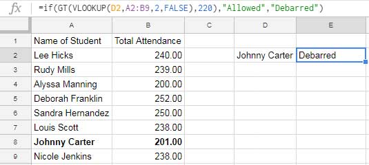
Suppose the data range A2:B9 contains student names in column A and their total attendance in column B. We can use VLOOKUP to find the attendance of a student whose name is entered in cell D2.
=VLOOKUP(D2, A2:B9, 2, FALSE)Now, what we aim to do with the IF and VLOOKUP combination is to determine if the attendance is greater than 220. If it is, the student is allowed to take the examination; otherwise, they are debarred.
Here’s how to achieve this using the comparison operator:
=IF(VLOOKUP(D2, A2:B9, 2, FALSE) > 220, "Allowed", "Debarred")
Alternatively, using equivalent functions:
=IF(GT(VLOOKUP(D2, A2:B9, 2, FALSE), 220), "Allowed", "Debarred"Controlling VLOOKUP Using a Checkbox
Do you want to enable/disable a VLOOKUP result in Google Sheets?
Navigate to the cell where you want to insert the checkbox. Click Insert > Tick box.
For instance, suppose cell D2 contains the checkbox, and the lookup range is A:B. The following formula entered in cell E2 will display the result when the checkbox is checked; otherwise, it will display blank.
=IF(D2, VLOOKUP("a", A:B, 2, FALSE), )


Hi Prashanth,
I followed up last time, but I think you missed it twice.
Can I have an update for this, or will you be able to reproduce it?
Thanks
Hi, Guenahel,
I left a comment within your Sheet because I was unsure about the problem you need to solve because of data in several tabs.
But I didn’t receive any response to my comment.
If I remember correctly, I have already solved two problems in that Sheet.
Please share a sample sheet with data ONLY in one tab and your expected result in another for further assistance. It can save my time.
If you want to solve several problems, It’s high time to hire someone.
Hi Prasanth,
Hope you are well.
Gentle follow up on my previous messages. I hope you can help me out. would really mean a lot for me
Hi, Guenahel,
Please share the sheet once again. I’ll check once free.
Hi Prashanth,
What you’ve done was pretty much amazing and helpful!
The data from the “General” Sheet should be pulled from the “Sample” sheet. If that work, the KVP Testing sheet will be flawless.
Here’s the Spreadsheet link for your reference: – URL removed by admin –
Hi, Guenahel,
That’s not matching your first requirement/query.
Having said that, please check the test_2 tab for a suggested formula.
Thank you.
I tried Query and using multi OR, but it doesn’t help much as it still filters unnecessary data that it shouldn’t.
Here’s the editable spreadsheet: – URL removed by admin –
Hi, Guenahel,
It’s difficult to manipulate data when there are merged cells.
So you should remove them physically or virtually.
I have virtually removed those merged cells and applied the Query.
Related:- How to Fill Merged Cells Down or to the Right in Google Sheets.
Check my tab “kvp testing” for the solution.
I’m trying to see how I can work out the Vlookup function and IF statement with my spreadsheet.
I want column C in the “Summary” Sheet to pull data from the “General” Sheet.
Here is my initial formula:
=VLOOKUP(A4,General!B2:M13,4)I’m trying to search that matches the Column “Summary A” on column “General B.”
When it matches, I want this to get the VA on column ” General D” only if column “General E” has a check or TRUE value.
Hi, Guenahel,
Thanks for your Sheet though it’s only viewable.
I’m suggesting you an array formula. Empty the range C3:C in the “Summary” tab.
Then insert the below Vlookup in C3.
=ArrayFormula(IFNA(vlookup(A3:A,filter(General!B2:D,General!E2:E=true),3,0)))Don’t copy it down.
Thank you so much! It worked!
Can you help me a bit more? There are still some things I can’t work out.
Is there any chance we can do screen sharing?
Hi, Guenahel,
Sorry! My time zone and busy schedule don’t allow me to do the same.
You can share a sample sheet as earlier with your notes in that.