If you use tick boxes to mark rows in Google Sheets, at some point you may need to VLOOKUP only in checkbox checked rows.

For example, we can use this to find or look up the price of only the available (checked) items in a table formatted as: item (text field), rate (numeric field), and availability (logical field, i.e., tick boxes).

What’s more — we can take it to the next level.

First, find the maximum or minimum rate of items in the ticked rows. Then use that value to look up the corresponding item.

It’s quite a simple task in Google Sheets because the FILTER function allows us to extract only checked rows from the table.

In this post, you’ll learn how to Vlookup only in checkbox checked rows in Google Sheets. I’ve also included the Max/Min example at the end.

Below you can find the sample data and a couple of examples.

Examples to Vlookup in Checkbox Checked Rows in a Table

1. Using FILTER within VLOOKUP in Google Sheets

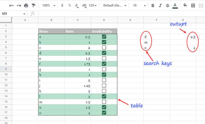
I have a three-column table with items, rates, and availability in the first, second, and third columns.

How to search for a few items and return their rate only if they are available? That’s the problem to solve.

Syntax:

VLOOKUP(search_key, range, index, [is_sorted])

• search_key (the items to search): F3:F5
• range: B2:D17 — Here, we want the checked rows. So we’ll use the following FILTER formula as the range to filter out unavailable (unchecked) items:
  FILTER(B3:C17, D3:D17)
• index: 2 (rate column number from the left of the filtered range)
• is_sorted: FALSE

Formula:

=IFNA(VLOOKUP(F3, FILTER($B$3:$C$17, $D$3:$D$17), 2, 0))

Insert it in cell G3 and copy it down for the other items (F4 and F5).

Alternatively, to search for multiple items in one go, wrap it with ARRAYFORMULA:

=ARRAYFORMULA(IFNA(VLOOKUP(F3:F5, FILTER($B$3:$C$17, $D$3:$D$17), 2, 0)))

2. Using a Logical Test Instead of FILTER

We can replace FILTER with IF in the above formula.

Range to use:

IF($D$3:$D$17, $B$3:$C$17)

Formula:

=ARRAYFORMULA(IFNA(VLOOKUP(F3:F5, IF($D$3:$D$17, $B$3:$C$17), 2, 0)))

Here also, I’ve used multiple search keys in one go, so ARRAYFORMULA is a must. Even if you use F3 instead of F3:F5, ARRAYFORMULA is still required because the IF logical test needs it.

VLOOKUP Max or Min in Checkbox Checked Rows in Google Sheets

Now, here’s a different scenario:

We’ll find the maximum or minimum rate in the checked rows and then use it as the search key in a Vlookup.

This can help us return the highest (or lowest) rate of available items in the table.

Step 1 – Find the Max or Min value
To get the maximum value from only checked rows:

=MAXIFS(C3:C17, D3:D17, TRUE)

This result will be our search key.

Step 2 – Prepare the range for Vlookup
Earlier, we used:

FILTER(B3:C17, D3:D17)

But here, that won’t work because we want to look up the rate (numeric field) as the search key, which means it must be in the first column of the lookup range.

So, reverse the column order:

FILTER(HSTACK(C3:C17, B3:B17), D3:D17)

Step 3 – Vlookup the item with the Max value

=VLOOKUP(MAXIFS(C3:C17, D3:D17, TRUE), FILTER(HSTACK(C3:C17, B3:B17), D3:D17), 2, 0)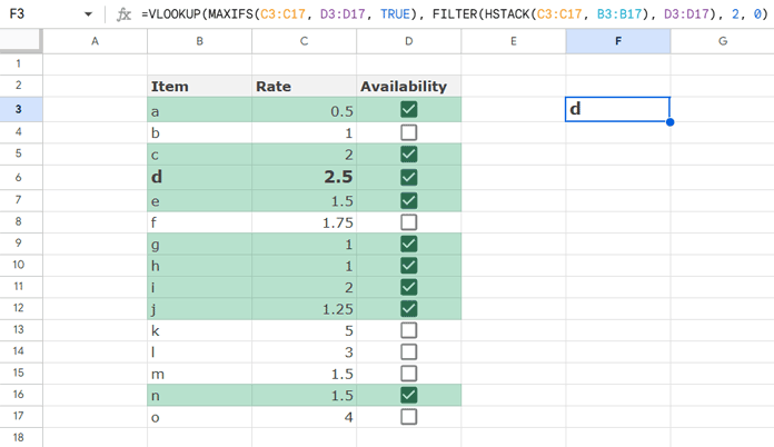

For Min instead of Max:
Just replace MAXIFS with MINIFS:

=VLOOKUP(MINIFS(C3:C17, D3:D17, TRUE), FILTER(HSTACK(C3:C17, B3:B17), D3:D17), 2, 0)

Thanks for reading. Enjoy your Google Sheets automation!

Resources

• How to Retrieve Multiple Results with VLOOKUP in Google Sheets
• VLOOKUP with Multiple Conditions in Google Sheets (Step-by-Step)
• Filter Specific Columns from VLOOKUP Results in Google Sheets
• Add and Use Check Marks or Tick Boxes in Google Sheets
• Create a List from Multiple Columns with Checked Tick Boxes in Google Sheets